Ijraset Journal For Research in Applied Science and Engineering Technology

Abstract

Financial Companies or firms try to determine if an individual or organization is worth lending specified amount of credit without any risk to its investors. If deemed eligible for it, they try to determine the risk associated (Probability of Default) with it. This Study compares Extreme gradient Boosting, Support Vector Machine, Naïve Bayesian, and Random Forest techniques for predicting the target variable efficiently with different strategies. This study tries to determine the risk using the person\'s assets, income, and various other parameters. Here, we are trying to calculate the home-credit risk factors using various parameters and compare various methods to try and determine which is more efficient and precise.

Introduction

I. INTRODUCTION

In modern era, many risks ranging from budgetary to defaulting on credit are associated to the financial firms [4]. To protect the investors of the institution from facing loss, financial firms try to determine the risk and probability of default of their clients. Financial Firms hold huge volumes of customer behavior related data from which they're unable to hit a judgement if an applicant may be defaulter or not. Credit risk analysis and management helps financial institutions in providing loans/credit to businesses or individuals while also overcoming risk which can occur due to various reasons like bank mortgages (or home loans), motorized vehicle purchase finances, credit card purchases, and installment purchases. To Protect the Investors of financial firms from facing financial loss in case of default, it is important to determine the risk associated with the credit [5].

In field of computer science, this problem is associated to classification machine learning. In this study, XGBoost, Naïve Bayesian, Random Forest, and Support Vector machine classifiers are used to predict the probability of loan default, which are later compared with each other to examine their reliability and efficiency. The use of machine learning algorithms has long raised various doubts [6]. The underlying fear is that algorithms may replace human which isn’t 100% reliable. In case of server crashes and denial of service, when heavily depended on machine can result in denial of service. However, these fears are not applicable which requires length process which go under multiple screening. The process of evaluating the probability of default should at least be semi-automated. This can help the financial institutions in eliminating foul play using personal connections [5].

A. Naïve Bayesian (NB)

Naïve Bayesian was initially generated using Bayes’ theorem. Bayes’ theorem determines the conditional probability of occurrence of event based on previously known knowledge. It consists of supervised statistical classifiers on assumption that all predictors are independent of each other [4]. For example, a vehicle may be considered to be a passenger vehicle if it has four wheels, can seat up to 6 people and are more than 4.7 m long, 1.7m wide, 2m high. Even if these features are dependent on one another they contribute to the probability that this vehicle is a passenger vehicle.

The formula of Bayes theorem is:

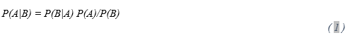
Here we are interested to find P(A|B), it is called as posterior probability and marginal probability of event P(A) is called the prior.

In this study, BernoulliNB from sklearn is used to implement Naïve Bayesian model. This model is used for multivariate models. It is suitable from discrete data. Discrete data is the data that take only categorical values. For example, “NAME_CONTRACT_TYPE” feature from the dataset used in this study has 2 values “Cash loans” and “Revolving loans”.

B. Random Forest (RF)

Random Forest uses numerous decision trees and aggregates them together to predict output classes for classification and regression problems. It is one of the supervised learning algorithm. As the name suggests it is a forest of Decision trees that is randomly created on data samples and these decision trees are further used for predictions. We know that more the number of trees, more robust is the forest, likewise more the number of decision trees, more precise the prediction model becomes [3]. After creating these trees, it gets each decision tree’s prediction and at last it selects the best suited solution using the voting. It assembles the result the then takes the average of the result b which it reduces overfitting because if which it is better than any single tree algorithms. 

The working of random forest can be explained in following steps:

1. Step-1: Select random n Subset or data points from the Dataset.
2. Step-2: Build decision trees with respect to the selected Subsets.
3. Step-3: Choose the number of decision trees N that you want to create
4. Step-4: Repeat 1 & 2.
5. Step-5: For each decision tree find the predictions for new data points, and then new data points are assigned to category that has the majority votes

C. Support Vector Machine (SVM)

Support vector machine has been previously applied to various financial application in field of time-series prediction and classification. Several previous studies have used SVM with various features and hyper parameters tuning for credit scoring algorithm [3]. SVM classifier prediction works by mapping data points to a high-dimensional feature space in order that data points are often categorized, even when the data is not linearly separable. A separator between the categories is calculated, then the data is transformed in such that the separator might be drawn as a hyperplane. After this process, the characteristics of new data can be used to predict the group to which a new record should belong.

D. Extreme Gradient Boosting (XGBoost)

Extreme Gradient Boosting is a scalable, gradient boosted decision tree machine learning algorithm. It provides the feature of parallel tree boosting. It was developed and designed as a research project at the University of Washington. It is being proved as the driving force for several industry-level application. XGBoost is a supervised machine learning algorithm which attempts to effectively predict response of response variable by combining combination of weaker machine learning techniques.

To predict new data point, XGBoost uses constructed trees or models to acquire all values to solve:

Here F2(x) is the prediction of the XGBoost Model [3].

II. METHODOLOGY

In this Study, credit risk associated with the loan is calculated using data analysis and mining. The dataset used to train the models is taken from Kaggle.

This dataset contains 346 attributes, some of which will be removed to avoid redundant data which is not required for this application. Here we will use pandas and sklearn python modules to accomplish tasks like data cleaning and normalization. Before using any dataset, we must make sure the data is unambiguous, and it doesn’t contain any missing data.

After Data Cleaning and Normalization, we will try and determine which is the better and efficient Prediction model for this use case with validation methods like Accuracy Score and Receiver operating characteristic (ROC). Few of the contenders for this supervised classification prediction model are Random Forest, XGBoost, Naïve bayesian and Support Vector machine. After selection of adequate supervised prediction model, we will try and determine the best features (parameters) to use for this model. To achieve this result, we will try the determine the correlation of feature associated with result.

The generic required steps involved for this analysis are mentioned below:

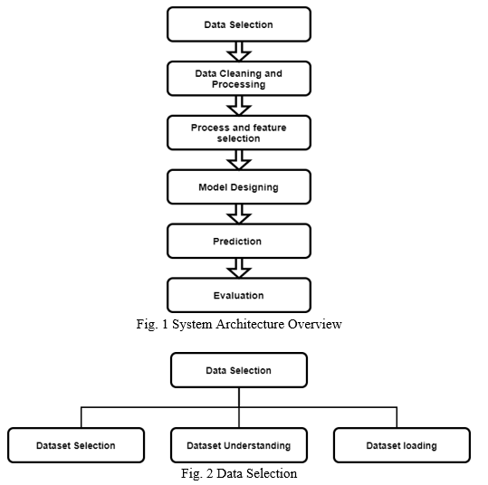
A. Data Selection and Dataset

When selecting the dataset for our evaluation and using it to train a prediction model, we must make sure it has no redundant data. We need to make sure the demographic audience for which this analysis is to be carried out is to be considered when selecting the dataset. For example, the dataset of popularity of a certain product will be different in USA as compared to India. Therefore, to get as precise results as possible, the dataset should be selected with extreme scrutiny.

Here for this study, the dataset we have used consists of multiple files aggregating to 220 total features with one Target column. The total amount of row is more than three hundred thousand. These datasets contain information like credit application details, previous application details, credit card balance, bank information, credit installment as well as assets [7].

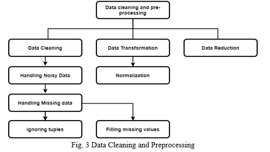
C. Data Cleaning and pre-processing

After selection of appropriate dataset for training of data, we need to make sure it does not contain any noisy or redundant data. If it does, we need to make sure to handle these problems before using it to train and test the prediction models. Python modules like Pandas, Scikit-learn, and NumPy will be used to address these issues. For example, null (empty), repeated values will be handled in this stage of project using data transformation techniques such as Normalization, Aggregation, and Generalization.

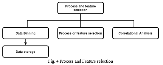
C. Process and Feature Selection

In Third stage, we must bifurcate independent and dependent attributes to build the prediction model. It is important to decide the features used to store and process the dataset to get result as it may affect the data privacy, efficiency, and precision of the final prediction model. In this stage, selection of method for data storage will also take place. Depending upon the volume and nature of dataset, we can use MySQL database, NoSQL, csv, or other methods to store the data. In this study, we have stored the dataset in csv files. The redundant attributes of dataset are removed to not affect our results and speed up processing time. These redundant attributes are the features which do not have any impact on result.

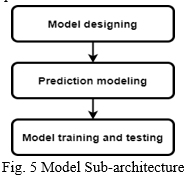
D. Model Designing

In this stage, we will classify the dataset into training and testing dataset. Generally, 80% to 70 % of the dataset is classified under training dataset while other is considered for testing. In this classification, the queries (rows) are selected on random, to not affect the integrity of the model. Random Forest, XGBoost, Naïve Bayesian and Support Vector machine (SVM) are the models to be compared for this application. The best compatible model for this application will be used to finalize the results.

E. Evaluation

Finally, the evaluation of the final model is conducted using Receiver operating characteristic (ROC) and Accuracy Score. Here, the trained models are tested using predict() or predict_proba() function based on the classification technique used. predict() function returns the predicted value the trained model infers output class from the previous experiences. While predict_proba() is used to infer class probability. predict_proba() is used to calculate to get more accurate ROC AUC score. Here, Accuracy Score and ROC Area under Curve is used to evaluate the models. It is as follows:

1. Accuracy Score: Accuracy Score is generally calculated using common metrics from confusion matrix. In this case the formula would be:

 However for this study the following function provided by sklearn.metrics is used:

metrics.accuracy_score(y_true,y_pred)

Here, y_true are the true/actual predictions and y_pred is the list of predicted values from the trained model.

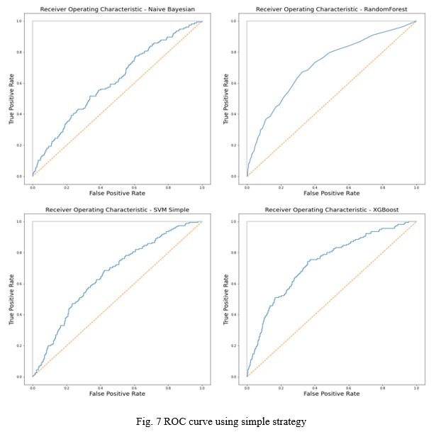
2. Receiver Operator Characteristic Curve: ROC presents how much a model is capable of distinguishing the output classes. Its value ranges from 1 to 0. A perfect predictor gives ROC AUC score of 1 and 0.5 score represents that the model’s prediction is as good as a guess. Anything below 0.5 means the model is reciprocating the result. ROC curve is plotted on True positive rate on Y-axis and False positive rate on X-axis. Which are calculated as:

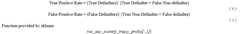
Here, y_true are the true/actual predictions and y_proba is the list of probability of value being true calculated by predict_proba() of the model.

III. APPROACH

We approached this problem in 3 specific strategies Simple, Iterative and Hybrid. These strategies are based on the techniques and algorithms used to implement the prediction model.

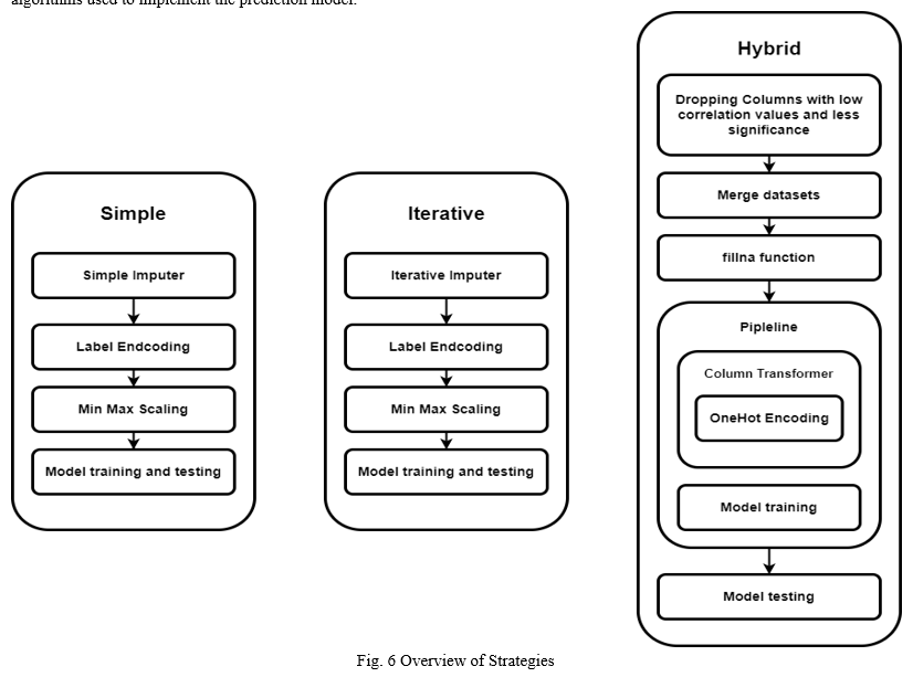
A. Simple

In Simple Strategy, the dataset is sparsely modified to preserve the integrity of data. This will result in the model fitting on original data. This is not the method that is ideally used to train models. However, to compare the varying results Simple Imputer to Iterative Imputer the dataset must not be drastically changed. The original dataset is sliced down to the size of 10k rows to test how the models perform with limited dataset. 121 Features from application_train dataset are used.

The dataset is later label encoded to convert any categorical data to Nominal numerical values. Related datasets were not used specifically because the goal of this strategy was to predict the outcome with least pre-processing and time required. After label encoding, min-max scaling was used to normalize data, to prevent values of high magnitude to affect the prediction ability of model.

This transformed dataset, is later fitted to Extreme Gradient Boosting, Bernoulli model in Naïve Bayesian, Support Vector Machine and Random Forest. They were later evaluated using Accuracy Score and ROC AUC score. Here, Random Forest model was trained with 100 estimators.

These are the results:

TABLE I

The time may defer on system basis. These tests were performed on AMD Ryzen 7 4800H and 16 GB DDR4 RAM.

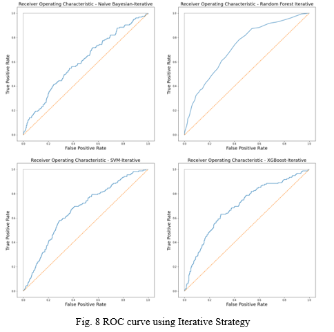
B. Iterative

The Iterative Strategy is same as Simple Strategy. However, here Iterative Imputer is used to handle missing values in the dataset. All the other parameters remain the same. Here, the dataset is still sliced down to 10k rows. 121 Features from application_train dataset are used.

TABLE II

The time may defer on system basis. These tests were performed on AMD Ryzen 7 4800H and 16 GB DDR4 RAM.

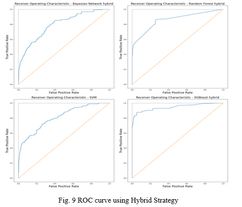
C. Hybrid

Hybrid Strategy uses the relational datasets provided to be merged to generate new dense dataset with high information value. Instead of stand-alone data cleaning processes, normalization, and model fitting, pipeline can be used to encapsulate data pre-processing, transformation, encoding, and prediction transform operations. In this case, Column transformer provided by scikit-learn was used along with the One Hot Encoding Algorithm. The encapsulated process along with high dense dataset result in better time complexity and efficiency.

Steps:

1. The relevant features from application_train are extracted by evaluating them using correlation value. The dataset includes features such as “OWN_CAR_AGE”,” WALLS_MATERIAL_MODE”, etc. These Features do not affect out response(target) variable in any way. Therefore, they are dropped.
2. This dataset will be used to merge related datasets provided by the source using “SK_ID_PREV”,”SK_ID_CURR”.
3. We will merge application_train, bureau, credit_card_balance, POS_CASH_balance, previous_applications and installments_payments datasets together to create dense dataset which actually modifies the final target.
4. Model Fitting

Dimensions of df are (372716,112)

The original merged dataframe is bifurcated to:

               X=df.drop([“SK_ID_PREV”,”SK_ID_CURR,” TARGET”], axis=1)

               Y=df[“TARGET”]

This X and Y dataframes are passed though train_test_split() to get X_train, X_test, y_train, y_test

We want to use this prediction model for deployment in real world hence the whole 3,72,716 rows of data are used to train the model. The exception was SVM model, where this dataset was sliced down to 100k rows, as compute time was more than 3 hours.

ColumnTransformer will be used along with OneHotEncoder to Encode categorical data in the whole dataset. This transformer will be encapsulated with the model in the pipeline to streamline the whole process during deployment.

               Pipeline will look like this:

pipeline = Pipeline (steps= [('transformer', transformer), ('model', model)])

5. After fitting the model with the dataset, it will be stored using joblib python module to the storage. This will be used in other application to predict default risk without training the model again and again. The pipeline will also make the encoding of dataset from raw data smooth and efficient.

6. Now, the model is evaluated using Accuracy score and ROC curve.

TABLE IIIIV

The time may defer on system basis. These tests were performed on AMD Ryzen 7 4800H and 16 GB DDR4 RAM.

IV. OUTCOME

1. Derived from the evaluation of models, we can conclude that for this dataset and Application the best performing technique is XGBoost (i.e. Extreme Gradient Boosting). It was the best performing model in all three strategies deployed. It was faster to compute and efficient on seen and unseen data. It was able to efficiently predict the unseen data with smaller dataset provided in first two strategies and was exceptional when using hybrid strategy.
2. Random Forest technique performed second best in our results, as ROC AUC score was above 0.7 in all cases. It was fast, efficient, and precise. We performed 100 iterations for this model to get best results we can get.  Random Forest ranks second in our analysis as it worked well with smaller as well as large dataset. However, it was second slowest model in this list.
3. SVM model was the slowest to fit, taking up to 10 hours on dataset of dimensions 300000x121.Fitting a SVM model on dataset having more than 100k (aka 1 lac) rows is not feasible. To fit the SVM model the original dataset was reduced to 100k, so it can be calculated in reasonable time. This reduced the time required but results were affected leading to underfitting due to shortage of data rows. It ranks third in this application.
4. Bernoulli technique from Naïve Bayesian (NB) was the most inconsistent on unseen data. ROC AUC score didn’t cross 0.7. However, it was fastest model to fit over the datasets [4].

TABLE VV

VI. FUTURE SCOPE

High Risk Liquidity assets of applicant can be considered into production of prediction model. Credit purpose can also affect the risk factor associated to Credit lending. Liability of a person can be considered in this model. There can also be use of Deep Learning algorithms instead of linear or polynomial statistical tests.

We can also test with different approaches to achieve a more desirable result, such as taking advantage of deep learning models and Neural Network. We can also consider datasets from different regions of the world to find more precise results.

Conclusion

As for Financial firms giving credit is associated with a high risk as they cannot gauge if a loan applicant may be a defaulter at a later stage or not. This Framework will help the Predict the Probability of Default so that financial firms will not face a much financial loss and increase the quantity of credits. Financial firms collect vast amount of information on their clients. This Information is used to determine the credit risk and probability of default associated with the client. Predictive analytic techniques like Random Forest, XGBoost gradient and Bayesian Network can be used to analyze and determine the risks (i.e. Probability of default) involved on credits, finances, and loans. Among all the techniques used, XGBoost was the standout in efficiency and effectiveness. It was moderately fast and predicted accurately even when it was provided with smaller dataset to work with. In conclusion, credit risk analysis is used to determine the creditworthiness of potential clients and their ability to repay credit. If the client is predicted under an acceptable level of default risk, the firm can recommend the approval of the application at the agreed conditions. The outcome of the credit risk analysis determines the probability of default of the borrower which will determine amount of credit he or she is eligible for.

References

[1] G. Caruso; S.A. Gattone; F. Fortuna; T. Di Battista. “Cluster Analysis for mixed data: An application to credit risk evaluation.” Elsevier Year: 2020 [2] Yiping Guo. \"Credit Risk Assessment of P2P Lending Platform towards Big Data based on BP Neural Network.” Elsevier Year: 2020 [3] Lkhagvadorj Munkhdalai; Tsendsuren Munkhdalai; Oyun-Erdene Namsrai; Jong Yun Lee; Keun Ho Ryu. “An Empirical Comparison of Machine-Learning Methods on Bank Client Credit Assessments.” Sustainability Year: 2019 (29 Jan 2019) [4] Germanno Teles; Joel J. P. C. Rodrigues; Ricardo A. L. Rabelo; Sergei A. Kozlov. “Artificial neural network and Bayesian network models for credit risk prediction.” Journal of Artificial Intelligence and Systems Year: 2020 [5] Mr Prashanta Kumar Behera. \"Credit Risk Analysis & Modeling: A Case Study\" IOSR-JEF. Volume 8, Issue 2 Ver. II (Mar. - Apr. 2017), PP 69-81. [6] Edward I Altman. Financial Ratios, Discriminant Analysis and the Prediction of Corporate Bankruptcy. The Journal of Finance, 23(4):589-609, 1968. [7] Dataset: https://www.kaggle.com/c/home-credit-default-risk/data

Copyright

Copyright © 2022 Gaurav Shinde, Shreyash Pawar, Rohit Albhar, Avaneesh Yadav, Mrs. Priyanka Patil. This is an open access article distributed under the Creative Commons Attribution License, which permits unrestricted use, distribution, and reproduction in any medium, provided the original work is properly cited.