Mathematical Modelling and Simulation of Suspension System in MATLAB/SIMULINK

Abstract

The main agenda of the following project is to help understand and appreciate principles and concepts of vibrations through an effective integration of software programs, MATLAB and SIMULINK, with theory. This further highlights the need for integration between mathematical analysis and engineering system design. The combination of MATLAB and SIMULINK is a powerful tool which adds a new dimension to research in vibrations systems control and to the instruction of vibrations courses since it has the promise of aiding us to understand much better the vibrations principle. There are five objectives that we aim in this project and they are listed as below: To present complex modelled imagination with calculated and specific measurements. To design and test machine controls of active suspension and supervisory logic for the function of closed loop feedback control. To help calculate the life of vehicle components by analyzing the road shocks transferred from the suspension to the chassis through simulation. To assist in the early development of prototype models in leading organizations. To describe the function of each component of suspension system.

Introduction

NOMENCLATURE

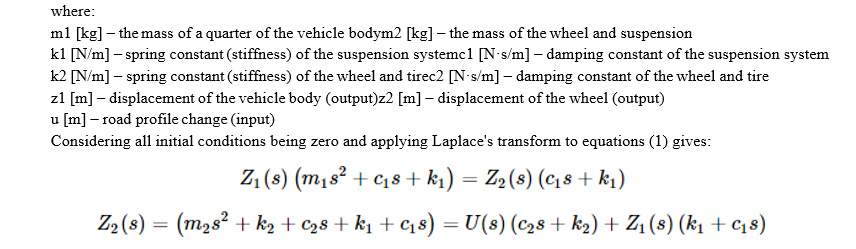
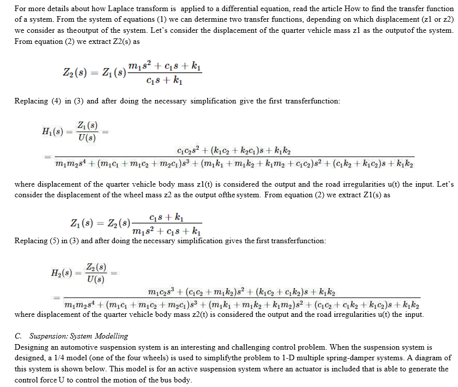
m1 [kg] – the mass of a quarter of the vehicle body

m2 [kg] – the mass of the wheel and suspension

k1 [N/m] – spring constant (stiffness) of the suspension system

c1 [N·s/m] – damping constant of the suspension system

k2 [N/m] – spring constant (stiffness) of the wheel and tire

c2 [N·s/m] – damping constant of the wheel and tire

z1 [m] – displacement of the vehicle body (output)

z2 [m] – displacement of the wheel (output) u [m] – road profile change (input)

A. Roll Movement Effect on Ride Comfort and Health

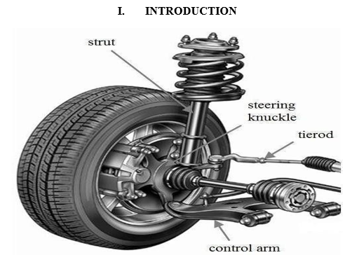
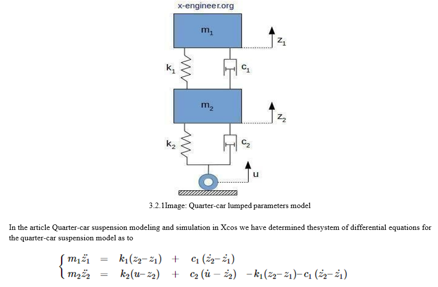
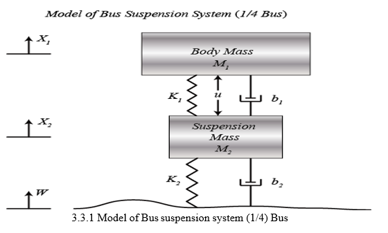
The suspension system's primary function is to maximize the overall performance of a vehicle as it cruises down the road. The suspension system also helps to absorb bumps in the road and provide a safe and comfortable ride The simplest model of a vehicle's suspension is called the quarter-car suspension model. The model consists of two mass bodies, quarter vehicle and wheel, and lumped parameters for stiffness and damping, for both suspension and tire.

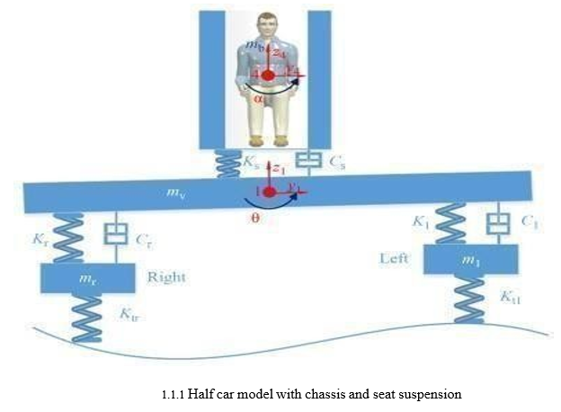
Generally, the conventional seat suspension design only considers the vertical vibration isolation, but heavy-duty vehicles, such as agricultural vehicles and construction vehicles, have severe roll vibration caused by uneven roads under the left and right tires of the vehicle, which will deteriorate the ride comfort significantly. Fig. 8.1 shows a half-car model with chassis and seat suspension, where ml, mr, mv, and mb are masses of the left tire, right tire, vehicle body, and driver body, respectively; K and C are the corresponding stiffness and damping parameters. The uneven road under the left and right tires will cause the vehicle’s vertical vibration, and at the same time, the roll vibration of vehicle chassis θ is generated. The vertical vibration and roll vibration will all be transferred to seat suspension. For normal road conditions, the magnitude of θ is small, thus, the roll vibration of driver body α is also small. Generally, by only controlling the vertical vibration, we can improve the ride comfort significantly. When the roll vibration magnitude is high, the driver's body looks like a mass on the top of an inverted pendulum; thus, the high magnitude lateral acceleration is caused by the rotary vibration:

(1.2.1) ay4=α¨r where is the roll acceleration of driver body; r is the distance from the center of driver body mass to its unknown rotary center; ay1 is the acceleration along the y4 axis of driver body caused by roll acceleration. ISO 2631-1 is a widely accepted standard to evaluate human exposure to WBV [26], which has defined the frequency weighted root mean square (FW-RMS) acceleration and the fourth power vibration dose value (VDV). The effect of vibration on driver health and ride comfort is dependent on the vibration frequency content.

The total vibration value of FW-RMS acceleration is calculated as

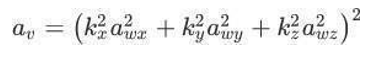
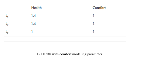
Where are awx, awy, and awz FW-RMS accelerations with respect to the three orthogonal axes;(Kx   Ky   KZ)   are multiplying factors which are defined in Table 1.1. with respect to health and ride comfort. The value of multiplying factors indicates that, with respect to the effect on ride comfort, the vibrations along three axes have the same weightings; but the longitudinal vibration (awx) and lateral vibration (awy) have more influence on health than vertical vibration (awz).

In this work, we only study the control of vibrations along with the z4 and y4 axes of the driver body. The vibration along the x4 axis of the driver’s body is more complicated, considering the existing effects of road slope, seat backrest, and feet on the floor; a similar control strategy could be applied.

II. LITERATURE REVIEW

In vehicles, the suspension system is applied to transmit the force and torsion between the wheel and the vehicle frame and buffer the impact force transmitted from the uneven road surface.[1] In [2], the active disturbance rejection control method is proposed to control the suspension system.

In [3], considering the actuator faults, an adaptive sliding mode control method is proposed to control the Markov jump suspension system.

In [4], and improved interval type-2 fuzzy logic control approach is designed to control the displacement of the suspension system.

In [5] and, the neural network is developed to approximate the unknown function in the active suspension, and some novel control schemes are proposed to control the suspension system.

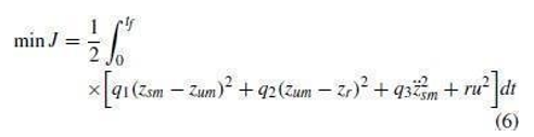
6. In this section, the optimal control objective is to improve handling stability and riding comfort. In the suspension system, the key variable related to the riding comfort is the vertical acceleration of the vehicle body. The key variables related to the handling stability are the suspension working space and the dynamic tire load. Therefore, the optimal control objective of the suspension system is defined as follows:

where q1, q2, q3, and rare are the weighting coefficients of the suspension working space, dynamic tire load, vertical acceleration, and control signal, respectively.

7. In this Work, one improved speed control algorithm of linear induction motors (LIMs) using sliding mode control (SMC) is firstly proposed. Then, an extended sliding mode load thrust observer (ESO) has been proposed to compensate for the sliding mode controller under the load thrust disturbance. Moreover, the SMC integrated with ESO is designed based on the direct thrust control (DTC) technique with space-vector modulation (SVM) to regulate the speed, flux, and thrust of the LIM. The output of the SMC is considered the reference thrust for the DTC based on space-vector modulation (DTC-SVM). A comparison between the proposed method and the conventional method with PI controllers is presented to illustrate the superiority of the proposed control method. Comprehensive simulation results have demonstrated that the proposed control scheme has a better transient control performance with fast and good speed tracking.

8. This Review technical note introduces the design of sliding mode control algorithms for nonlinear systems in the presence of hard inequality constraints on both control and state variables. Relying on general results on minimum-time higher-order sliding mode for unconstrained systems, a general order control law is formulated to robustly steer the state to the origin while satisfying all the imposed constraints. Results on minimum-time convergence to the sliding manifold, as well as on the maximization of the domain of attraction, are analytically proved for the first-order and second-order sliding mode cases. A general result is presented regarding the domain of attraction in the general order case, while numerical results on the estimation of the domain of attraction and on minimum-time convergence are discussed for the third-order case, following a procedure applicable to a sliding mode of any order.

9. in this work, A neural network (NN) adaptive control design problem is addressed for a class of uncertain multi-input-multi-output (MIMO) nonlinear systems in block-triangular form. The considered systems contain uncertainty dynamics and their states are enforced subject to bounded constraints as well as the couplings among various inputs and outputs are inserted in each subsystem. To stabilize this class of systems, a novel adaptive control strategy is constructively framed by using the backstepping design technique and NNs. The novel integral barrier Lyapunov functional (BLFs) are employed to overcome the violation of the full state constraints. The proposed strategy can not only guarantee the boundedness of the closed-loop system and the outputs are driven to follow the reference signals, but also can ensure all the states remain in the predefined compact sets. Moreover, the transformed constraints on the errors are used in the previous BLF, and accordingly, it is required to determine clearly the bounds of the virtual controllers. Thus, it can relax the conservative limitations in the traditional BLF-based controls for the full state constraints

10. This Review proposes adaptive control designs for vehicle active suspension systems with unknown nonlinear dynamics (e.g., nonlinear spring and piece-wise linear damper dynamics). Adaptive control is first proposed to stabilize the vertical vehicle displacement and thus improve the ride comfort and guarantee other suspension requirements (e.g., road holding and suspension space limitation) concerning the vehicle safety and mechanical constraints. An augmented neural network is developed to online compensate for the unknown nonlinearities, and a novel adaptive law is developed to estimate both NN weights and uncertain model parameters (e.g., sprung mass), where the parameter estimation error is used as a leakage term superimposed on the classical adaptations

11. This paper proposes an adaptive backstepping control strategy for vehicle active suspensions with hard constraints. An adaptive backstepping controller is designed to stabilize the attitude of the vehicle and meanwhile improve ride comfort in the presence of parameter uncertainties, where suspension spaces, dynamic tire loads, and actuator saturations are considered as time-domain constraints. In addition to spring nonlinearity, the piecewise linear behavior of the damper, which has different damping rates for compression and extension movements, is taken into consideration to form the basis of accurate control. Furthermore, a reference trajectory is planned to keep the vertical and pitch motions of the car body stabilized in a predetermined time, which helps adjust accelerations accordingly to high or low levels for improving ride comfort. Finally, a design example is shown to illustrate the effectiveness of the proposed control law.

A.  Gap Analysis

In the existing work, many simulation analyses are performed only by using MATLAB/Simulink software. In this article, by using the MATLAB/Simulink software, a collaborative simulation platform for vehicle control is developed. Simulation of using quarter car model is a special vehicle dynamics simulation software in the vehicle industry. In the developed collaborative simulation platform, the actual vehicle model of Matlab software is utilized as the controlled plant, which can better verify the effectiveness of the controller

B.  Problem Statement

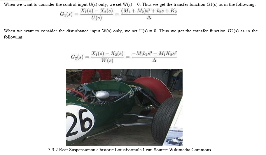
This model allows you to simulate the effects of changing the suspension damping and stiffness, thereby investigating the tradeoff between comfort and performance. In general, racing cars have very stiff springs with a high damping factor.

C.  Objectives

The main objective of the following project, given to our students in vibration class, is to help them understand and appreciate principles and concepts of vibrations through effective integration of software programs, MATLAB, and SIMULINK, with theory. This further highlights the need for integration between mathematical analysis and engineering system design.

After the assignment of the following project, it became increasingly evident to the Authors of this article that the combination of MATLAB and SIMULINK is a powerful tool that adds a new dimension to research in vibrations systems’ control and to the instruction of vibrations courses since it has the promise of aiding to understand much better the Vibrations principles. Our students showed a deep understanding of such principles, as a result.

III. TYPES OF SUSPENSIONS

A.  What Are the Different Types Of Suspensions

8 Types of Car Suspensions:

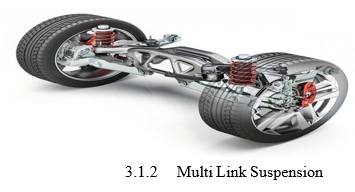
• Multi-Link Suspension.
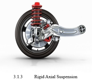
• Rigid Axle Suspension.
• Macpherson Suspension.
• Double Wishbone Suspension.
• Independent Suspension.
• Rigid suspension – Leaf Spring.
• Trailing Arm Suspension.
• Air Suspension.

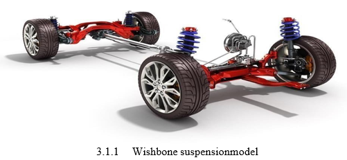
The Double Wishbone suspension also has an independent design, so the turning angle and suspension movement will not affect the geometry angle, because the angle will remain constant. The Double Wishbone suspension has drawbacks due to the fairly large space it requires. On top of that, when you want to replace a shock breaker or shock absorber, the disassembly process takes a long time. This suspension is fairly easy to get damaged in its parts, such as broken ball joint at the bottom or top, lo tie rod, and end tier rod. To avoid various damage to the car, you can do spooring regularly.

1.  Multi-link Suspension

Multi-Link is a suspension developed by Double Wishbone and Multi-Link into a suspension that has a fairly complicated construction design because it has separate parts that are held together by joints. This suspension also has component ends that pivot on two sides of the arm. Construction is made by manipulating the direction of the force that will be received by the wheel. Multi-Link is a type of suspension that has quality grip and with this suspension, controlling the car becomes easier. The Multi-Link suspension also has many variations. If this suspension is damaged, then the replacement process takes a long time and the spare parts are still rare, so the price is relatively more expensive than other suspensions.

2. Rigid Axle Suspension

Is usually placed at the rear of the car. The main feature of this suspension is its wheels on the rear left and right. The two wheels are connected into one axle which is commonly referred to as the axle. The rigid axle suspension has 2 models at once, namely the Axle Rigid model which is equipped with leaf springs, and the Axle Rigid model which is equipped with a coil spring or often referred to as a spring.

 

 

This suspension has fairly good quality and can be applied to various types of cars. It is fairly simple because it can work with just one solid piece and is equipped with 2 springs. The axle rigid is also considered a strong suspension, so it can support large loads stably, making it suitable for various types of large cars. Suspension can help dampen the vibrations or shocks that occur when you are on a road that is uneven or tends to be bumpy. With a good-quality suspension car, you can stay seated without any disruption. The suspension is not only useful to help reduce vibrations when the car is driving but can make handling safer and let the car can run stably on the road. With its very significant use, of course, the suspension is a must-have component in a car and it must get extra care. Now, there are many types of cars around the world and this makes a variety of suspension types available. Even the use of suspensions in each car brand is always different, due to the large number of quality suspensions. Differentiating the type of suspension in each car brand is certainly a way to balance the type of car. At least several types of suspension are widely popular and used in cars produced nowadays.

3. Macpherson Suspension

 

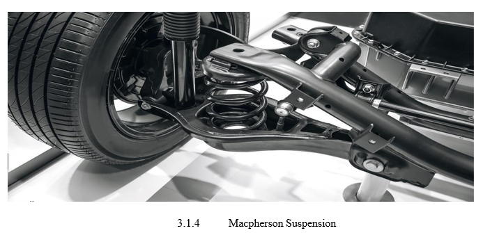
Macpherson is a suspension whose name is taken from its inventor, Earle Macpherson. Lots of cars around the world use Macpherson suspension. Many automotive manufacturers like this suspension, because it has an affordable price and also has fairly simple components. The Macpherson suspension has an upright shape and is supported by shock absorbers which are used as the center point of the corner caster in the car. This suspension is also very easy to obtain because it’s distributed widely. The disadvantage of Macpherson’s suspension is that it is less able to receive loads and the tilt angle always changes when the car is turned or turns, this makes the tires less able to grip the road asphalt properly.

4. Double Wishbone Suspension

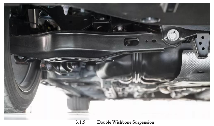
Double Wishbone is a type of suspension that has 2 arms that support the suspension system, namely the upper and lower arms. With this suspension, the car can run stably.

a. Independent Suspension

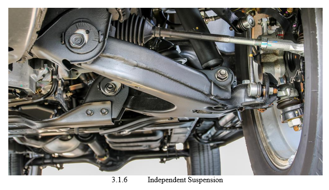
Is a specially designed suspension because the right and left wheels at the rear are not connected directly but instead by axle joints If the rear wheel steps on a hole, of course, the car will not rock and this is because only the left suspension moves. Independent suspension is indeed widely used in luxury cars. The independent suspension has a more complex construction and the axle movements are mutually independent. This suspension is also equipped with two flexible joints. This type of suspension is still fairly expensive, so its use is mostly in luxurious cars. You can also feel the comfort of the Independent Suspension when driving the Wuling Cortez CT Type S. This family car from Wuling offers comfort through Independent Suspension on the rear wheels. Of course, not only drivers but passengers can also feel comfortable sitting at the back seat of Wuling Cortez CT City Type S.

5. Rigid Suspension - Leaf Spring

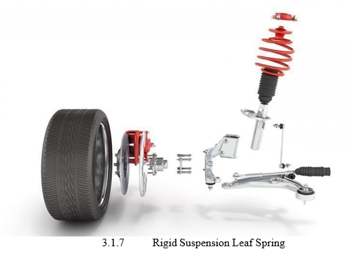
Rigid – Leaf spring is one type of suspension that is widely applied in cars circulating in Indonesia and is mostly used in commercial type cars or old type cars. This suspension is usually used at the rear of the car because this suspension is stiff. This suspension has a fairly simple and simple construction. This type of suspension usually consists of an Axle Housing that is intentionally tied using a U-Bolt already attached to the frame. Cars that use this suspension usually have a fairly high level of resistance.

6. Trailing Arm Suspension

 

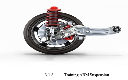
Trailing Arm is a type of suspension whose instructions are almost the same as 3 Links – Rigid, even though the working system is very different. The way it works is also different from the 3 Links – Rigid or other types of suspension. The Trailing Arm suspension has connected from the right side to the left. This type of suspension is usually placed at the back of the car.

7. Air Suspension

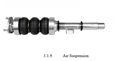
Is one of the developed suspensions that has excellent performance, so this type of suspension is widely used in luxury cars. Even in luxury cars, the car’s suspension can be adjusted using a computer and this allows the adjustment to be done properly. The drawback of this suspension is that it has a very complicated construction when compared to other types of suspension. Not only that, but this suspension also has a very expensive price. Those are the eight types of car suspensions that exist today. Hopefully, this information can add to your automotive knowledge!

B.  Constructional Features of Suspension

There exists a vast classification of the suspension system, though all suspensions have common integral elements:

• Details responsible for elasticity;
• Details that spread force direction;
• Absorbing elements;
• Mountings;
• Components that stabilize sway steadiness.

Automobile suspension is a complex of mechanisms that make up chassis together and perform the function of a link connecting the car body and road surface.

Vehicles went without suspensions for quite a long time. It was simply unnecessary at slow speeds. However, with the course of automobile industry development, increasing road quality and transporting speed there arose the need to increase transportation comfort. Let’s have a closer look at what is the suspension system, what are its construction features, functions and what types of suspension exist. Some background: how the first suspension appeared and construction improvement The first suspension looked rather primitive – details on long belts of leather or chains. When movement speed increased is tangibly decreased jumps and smoothened fluctuations of the compartment. Such a system was installed on caroches and post coaches. The scheme of modern suspension with bearings and elastic elements was developed by O. Elliott from England at the beginning of the 19th century. They used steel and wood for making shock absorbers. However, the item was still far from perfect and often broke on rough roads. They managed to overcome this defect as the metallurgy industry developed and made the suspension more rigid and load-resistant. Noticeably, such construction is still used in load-carrying trucks. The story of modern automotive suspension started in 1898. A French company named Deauville first used McPherson knee-action suspension with immovable bearings in a passenger car. Shock absorbers were first installed on automobiles in 1901. Mr. Mors, a Frenchman, installed them on a racing car as an experiment and in that very year, the race car driven by a racer A. Fourier won the race Paris-Berlin. Later in 1906 carriage springs were replaced by cylinder springs. Then during the 30s-50s construction engineers from all over the world worked on suspension improvement and tried each and every scheme of its construction and installation. From among all tested construction types the optimum ones were selected which are used by this day. Nowadays most passenger cars use suspensions of three types – independent construction, independent on double cross-installed levers, and semi-dependent with a torsion beam.

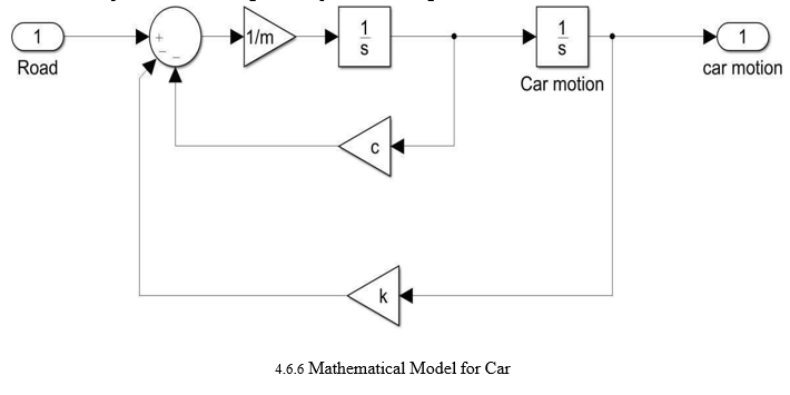
1. Quarter Car Suspension Model Transfer Function

The dynamics of the suspension of a vehicle can be analyzed by running simulations through a mathematical model. The simplest model of a vehicle’s suspension is called the quarter-car suspension model. The model consists of two mass bodies, quarter vehicle and wheel, and lumped parameters for stiffness and damping, for both suspension and tire.

Model and simulate dynamic system behavior with MATLAB, Simulink, Stateflow, and Simscape. Modeling is a way to create a virtual representation of a real-world system that includes software and hardware. Common representations for system models include block diagrams, schematics, and state diagrams. Simulink provides a graphical editor, customizable block libraries, and solvers for modeling and simulating dynamic systems. It is integrated with MATLAB®, enabling you to incorporate MATLAB algorithms into models and export simulation results to MATLAB for further analysis. Simulink is a tool for controls engineers to torture embedded systems engineers with huge volumes of hard-to-read generated C. ;) Simulink and it's add-ons are widely used in almost every engineering discipline.

There are three (3) types of commonly used simulations:

• • Live: Simulation involving real people operating real systems. Involve individuals or groups.
  • Virtual: Simulation involving real people operating simulated systems.

 

• • Constructive: Simulation involving simulated people operating simulated systems.

Need for simulation

Simulation modeling solves real-world problems safely and efficiently. It provides an important method of analysis that is easily verified, communicated, and understood. Across industries and disciplines, simulation modeling provides valuable solutions by giving clear insights into complex systems.

???????A.  Road Geometry

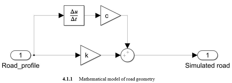
B. Geometric Design of Roads

The geometric design of roads is the branch of highway engineering concerned with the positioning of the physical elements of the roadway according to standards and constraints. The basic objectives of geometric design are to optimize efficiency and safety while minimizing cost and environmental damage. The geometric design also affects an emerging fifth objective called "livability," which is defined as designing roads to foster broader community goals, including providing access to employment, schools, businesses, and residences, accommodating a range of travel modes such as walking, bicycling, transit, and automobiles, and minimizing fuel use, emissions, and environmental damage.

Geometric roadway design can be broken into three main parts: alignment, profile, and cross- section. Combined, they provide a three-dimensional layout for a roadway. The alignment is the route of the road, defined as a series of horizontal tangents and curves. The profile is the vertical aspect of the road, including crest and sag curves, and the straight grade lines connecting them. The cross-section shows the position and number of vehicle and bicycle lanes and sidewalks, along with their cross slope or banking. Cross-sections also show drainage features, pavement structure, and other items outside the category of geometric design.

Symbols used

• BVC = beginning of vertical curve
• EVC = end of vertical curve
• g1 = initial roadway grade, expressed in percent
• g2 = final roadway grade expressed in percent
• A = absolute value of the difference in grades (initial minus final), expressed in percent
• h1 = height of eye above the roadway, measured in meters or feet
• h2 = height of an object above the roadway, measured in meters or feet
• L = curve length (along the x-axis)
• PVI = point of vertical interception (intersection of initial and final grades)
• S = headlight sight distance
• Tangent elevation = elevation of a point along the initial tangent
• x = horizontal distance from BVC
• Y (offset) = vertical distance from the initial tangent to a point on the curve
• Y′ = curve elevation = tangent elevation offset .

???????C.  SAG Curves

Sag vertical curves are curves that, when viewed from the side, are concave upwards. This includes vertical curves at valley bottoms, but it also includes locations where an uphill grade becomes steeper, or a downhill grade becomes less steep.

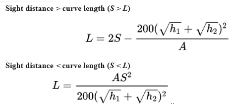
The most important design criterion for these curves is headlight sight distance.[2] When a driver is driving on a sag curve at night, the sight distance is limited by the higher grade in front of the vehicle. This distance must be long enough that the driver can see any obstruction on the road and stop the vehicle within the headlight sight distance. The headlight sight distance (S) is determined by the angle of the headlight and the angle of the tangent slope at the end of the curve. By first finding the headlight sight distance (S) and then solving for the curve length (L) in each of the equations below, the correct curve length can be determined. If the S < L curve length is greater than the headlight sight distance, then this number can be used. If it is smaller, this value cannot be used. Similarly, if the S>L curve length is smaller than the headlight sight distance, then this number can be used. If it is larger, this value cannot be used.

UNITS	Sight       Distance Length (S<L)		<	Curve	Sight       Distance        >                Curve Distance (S>L)
Metrics (s in meters)	L=	2 ???????? 120+3.5 ????			L=2S-       120+3.5???? ????
US Customary (S in Feet)	L=	2 ???????? 400+3.5 ????			L=2S-???? = 400+3.5???? ????

1. Crest Curves

Crest vertical curves are curves which, when viewed from the side, are convex upwards. This includes vertical curves at hill crests, but it also includes locations where an uphill grade becomes less steep, or a downhill grade becomes steeper. The most important design criterion for these curves is stopping sight distance.[2] This is the distance a driver can see over the crest of the curve. If the driver cannot see an obstruction in the roadway, such as a stalled vehicle or an animal, the driver may not be able to stop the vehicle in time to avoid a crash. The desired stopping sight distance (S) is determined by the speed of traffic on a road. By first finding the stopping sight distance (S) and then solving for the curve length (L) in each of the equations below, the correct curve length can be determined. The proper equation depends on whether the vertical curve is shorter or longer than the available sight distance. Normally, both equations are solved, then the results are compared to the curve length.

US standards specify the height of the driver’s eye is defined as 1080 mm (3.5 ft) above the pavement, and the height of the object the driver needs to see as 600 mm (2.0 ft), which is equivalent to the taillight height of most passenger cars For bicycle facilities, the cyclist's eye height is assumed to be at 1.4 m (4.5 ft), and the object height is 0 inches since a pavement defect can cause a cyclist to fall or lose control.

???????2.  Alignment

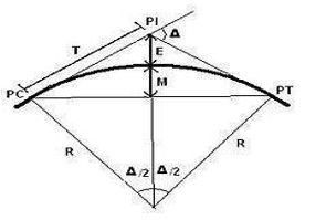
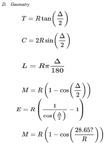
Horizontal alignment in road design consists of straight sections of road, known as tangents, connected by circular horizontal curves.[2] Circular curves are defined by radius (tightness) and deflection angle (extent). The design of a horizontal curve entails the determination of a minimum radius (based on speed limit), curve length, and objects obstructing the view of the driver.

Using AASHTO standards, an engineer works to design a road that is safe and comfortable. If a horizontal curve has a high speed and a small radius, increased superelevation (bank) is needed in order to assure safety. If there is an object obstructing the view around a corner or curve, the engineer must work to ensure that drivers can see far enough to stop to avoid an accident or accelerate to join traffic.

Terminology

• BC = beginning of curve
• EC = end of curve
• R = radius
• PC = point of curvature (point at which the curve begins)
• PT = point of tangent (point at which the curve ends)
• PI = point of intersection (point at which the two tangents intersect)
• T = tangent length
• C = long chord length (straight line between PC and PT)
• L = curve length
• M = middle ordinate, now known as HSO – horizontal sightline offset (distance from the sight-obstructing object to the middle of the outside lane)
• E = external distance
• fs= coefficient of side friction
• u= vehicle speed
• ?= deflection Angle

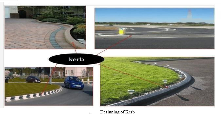
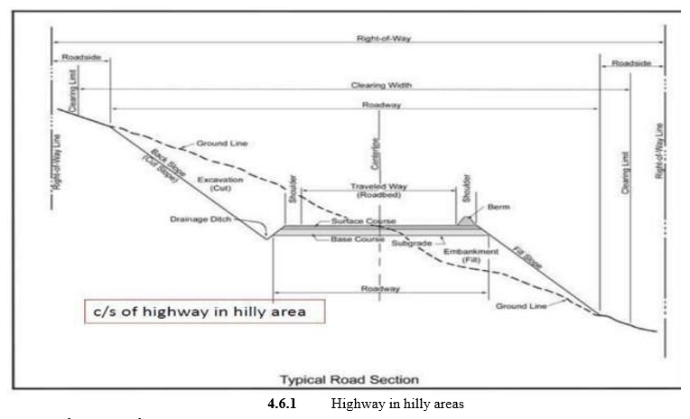
1. Cross Section: The cross-section of a roadway can be considered a representation of what one would see if an excavator dug a trench across a roadway, showing the number of lanes, their widths, and cross slopes, as well as the presence or absence of shoulders, curbs, sidewalks, drains, ditches, and other roadway features. The cross-sectional shape of a road surface, in particular in connection to its role in managing runoff, is called "crown".
2. Lane Width: The selection of lane width affects the cost and performance of a highway. Typical lane widths range from 3 meters (9.8 ft) to 3.6 meters (12 ft). Wider lanes and shoulders are usually used on roads with higher speed and higher volume traffic, and with significant numbers of trucks and other large vehicles. Narrower lanes may be used on roads with lower speed or lower volume traffic. As lane width decreases, traffic speed diminishes, and so does the interval between vehicles; throughput is maximal at 18 miles per hour km/h). Narrow lanes cost less to build and maintain. They lessen the time needed to walk across and reduce stormwater runoff. Pedestrian volume declines as lanes widen, and intersections with narrower lanes provide the highest capacity for bicycles.
3. Safety: On rural roads, narrow lanes may experience higher rates of run-off-road and head-on collisions.[citation needed] In urban settings, both narrow (less than 2.8 metres (9 ft 2 in)) and wide (over 3.1 meters (10 ft)) lanes increase crash risks, which are lowest at a width of 3.0 to 3.1 meters (9.8 to 10.2 ft). Lanes wider than 3.3~3.4m (10.8-11.2 ft)) are associated with 33% higher impact speeds and more severe collisions, as well as higher crash rates. Carrying capacity is also maximal at a width of 3.0 to 3.1 meters (9.8 to 10.2 ft), both for motor traffic and for bicycles. [10] Thus, safety and capacity on most roads are optimal if lane widths are reduced to as little as 10 ft (3.0 m).
4. Cross Slope: See also: Cant (road/rail) Steeper cants or cambers are common on residential streets, allowing water to drain into the gutter Cross slope describes the slope of a roadway perpendicular to the centerline. If a road were completely level, water would drain off it very slowly. This would create problems with hydroplaning, and ice accumulation in cold weather. In tangent (straight) sections, the road surface cross slope is commonly 1—2% to enable water to drain from the roadway. Cross slopes of this size, especially when applied in both directions of travel with a crown point along the centerline of a roadway are commonly referred to as "normal crown" and are generally unnoticeable to traveling motorists. In curved sections, the outside edge of the road is super elevated above the centerline. Since the road is sloped down toward the inside of the curve, gravity draws the vehicle toward the inside of the curve. This causes a greater proportion of centripetal force to supplant the tire friction that would otherwise be needed to negotiate the curve.

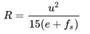
Superelevation slopes of 4 to 10% are applied to aid motorists in safely traversing these sections while maintaining vehicle speed throughout the length of the curve. An upper bound of 12% was chosen to meet the demands of construction and maintenance practices, as well as to limit the difficulty of driving a steeply cross-sloped curve at low speeds. In areas that receive significant snow and ice, most agencies use a maximum cross slope of 6 to 8%. While a steeper cross slope makes it difficult to traverse the slope at low speed when the surface is icy, and when accelerating from zero with warm tires on the ice, a lower cross slope increases the risk of loss of control at high speeds, especially when the surface is icy. Since the consequence of high-speed skidding is much worse than that of sliding inward at a low speed, sharp curves have the benefit of greater net safety when designers select up to 8% superelevation, instead of 4%.[citation needed] A lower slope of 4% is commonly used on urban roadways where speeds are lower, and where a steeper slope would raise the outside road edge above adjacent terrain. The equation for the desired radius of a curve, shown below, takes into account the factors of speed and superelevation (ethe ). This equation can be algebraically rearranged to obtain desired rate of superelevation, using the input of the roadway's designated speed and curve radius.

???????E.  Safety Effects of Road Geometry

1. Design Consistency

Collisions tend to be more frequent in locations where a sudden change in road character violates the driver's expectations. A common example is a sharp curve at the end of a long tangent section of the road. The concept of design consistency addresses this by comparing adjacent road segments and identifying sites with changes the driver might find sudden or unexpected. Locations with large changes in the predicted operating speed are likely to benefit from additional design effort. A horizontal curve with a significantly smaller radius than those before it may need enhanced curve signs. This is an improvement on the concept of design speed, which only sets a lower limit for geometric design. In the example given above, a long tangent followed by a sharp curve would be acceptable if a 30 mph design speed was chosen. Design consistency analysis would flag the decrease in operating speed at the curve.

???????2.  Safety Effects of alignment

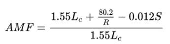
The safety of a horizontal curve is affected by the length of the curve, the curve radius, whether spiral transition curves are used, and the superelevation of the roadway. For a given curve deflection, crashes are more likely on curves with a smaller radius. Spiral transitions decrease crashes, and insufficient superelevation increases crash. A safety performance function to model curve performance on two-lane roads is

Where,

AMF = Accident modification factor, a multiplier that describes how many more crashes are likely to occur on the curve compared to a straight road

Lc = Length of the horizontal curve in miles. R = Radius of the curve in feet.

S = 1 if spiral transition curves are present

= 0 if spiral transition curves are absent

???????3.  Safety Effects of cross-section

Cross slope and lane width affect the safety performance of a road. Certain types of crashes, termed "lane departure crashes", are more likely on roads with narrow lanes. These include run- off-road collisions, sideswipes, and head-on collisions. For two-lane rural roads carrying over 2000 vehicles per day, the expected increase in crashes is

Lane Width	Expected increase in crashes
is 12 feet (3.7m)	0%
11 feet (3.4m)	5%
10 feet (3.0m)	30%
9 feet (2.7m)	50%

The effect of lane width is reduced on urban and suburban roads and low volume roads. Insufficient superelevation will also increase the crash rate. The expected increase is shown below

Suppper elevation deficiency	Expected increase in crashes
	Cars	Heavy trucks
<0.01	0%	<5%
0.02	6%	10%
0.03	9%	15%
0.0.4	12%	20%
0.0.5	15%	25%

???????F.  Geometric Design for Highway

SL.no	Class of road	Width of the carriageway in ‘M’
1	Single lane	3.75
2	Two-lane without raised Kerbs	7.0
3	Two lanes with raised Kerbs	7.5
4	Intermediate lane	5.5
5	Multilane Pavement	3.5/lane

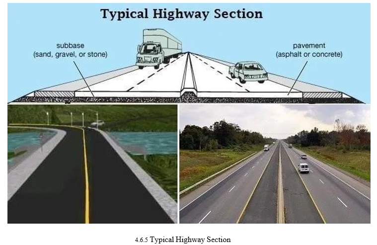
Highway cross-section elements

• Carriageway.
• Shoulders.
• Roadway width.
• Right of way.
• Building line.
• Control line.
• Medin.
• Camber/ cross slope
• Crown. Side slope.
• Kerbl. Guard rail.
• Side drain.
• Other facilities

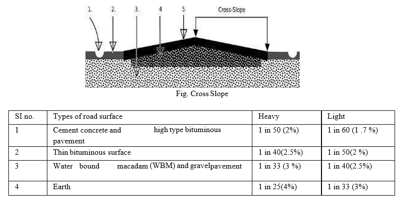
1. Cross Slope or Camber

It is the slope provided to the road surface in the transverse direction to drain off the rainwater from the road surface.

 

 

 

• To prevent the entry of surface water into the sub-grade soil through the pavement.
• To prevent the entry of water into the bituminous pavement layer.
• To remove the rainwater from the pavement surface as quickly as possible and to allow the pavement to get dry soon after the rain.
• It is expressed as a percentage or 1 V: N h.
• It depends on the pavement surface and amount of rainfall.-Shape of the cross slope:- Parabolic shape(fast-moving vehicle).- Straight line. - Combination of a parabolic and straight line.

2. Importance of geometric design

The geometric design of a highway deals with the dimensions and layout of visible features of the highway such as alignment, sight distance, and intersection. The main objective of highway design is to provide optimum efficiency in traffic operation with maximum safety at a reasonable cost.

The geometric design of highways deals with the following elements

• Cross-section elements
• Sight distance considerations
• Horizontal alignment details
• Vertical alignment details
• Intersection element

3. Design controls and criteria

• Design Speed
• Topography
• Traffic factors
• Design hourly volume and capacity
• Environmental and other factors

Design speed: different speed standards have been assigned for different classes of road. Design speed may be modified depending upon the terrain conditions.

a. Topography

• Plain Terrain <10%
  • Rolling terrain 10-25%
  • Mountainous terrain 25-60%
  • Steep terrain >60%

b. Traffic Factor

• Vehicular characteristics and human characteristics of road users.
• Different vehicle classes have different speed and acceleration characteristics, different dimensions, and weights.
• The human factor includes the physical, mental and psychological characteristics of drivers and pedestrians.

c. Design hourly volume and capacity

• Traffic flow fluctuating with time
• Low value during off-peak hours to the highest value during the peak hour. It is uneconomical to design the roadway for peak traffic flow.

d. Environmental Factors

• Aesthetics
• Landscaping
• Air pollution
• Noise pollution

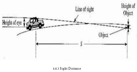
e. Sight Distance: Sight distance available from a point is the actual distance along the road surface, in which a driver from a specified height above the carriageway has visibility of stationary or moving objects. OR It is the length of road visible ahead to the driver at any instance

f. 

f. Types of Sight Distance

• Stopping or absolute minimum sight distance (SSD)
• Safe overtaking or passing sight distance (OSD)
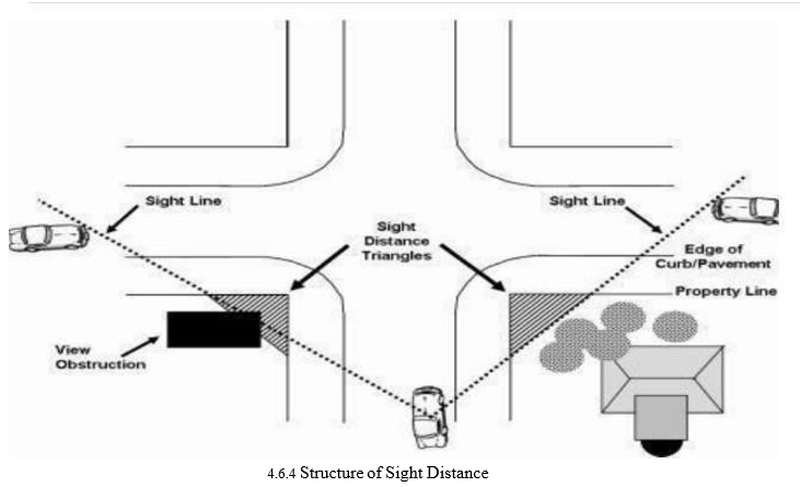
• Safe sight distance for entering uncontrolled intersection
• Intermediate sight distance
• Headlight sight distance

g. Stopping Sight Distance: The minimum sight distance available on a highway at any spot should be of sufficient length to stop a vehicle traveling at design speed, safely without collision with any other obstruction.

h. Overtaking Sight Distance: The minimum distance open to the vision of the driver of a vehicle intending to overtake a slow vehicle ahead with safety against the traffic in opposite direction is known as the minimum overtaking sight distance (OSD) or the safe passing sight distance.

i. Stopping Sight Distance

SSD is the minimum sight distance available on a highway at any spot having sufficient length to enable the driver to stop a vehicle traveling at design speed, safely without collision with any other obstruction.

It depends on

1. Feature of the road ahead
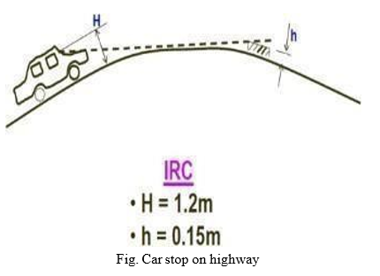
2. Height of driver’s eye above the road surface(1.2m)c. Height of the object above the road surface (0.15m).

Criteria for measurement

1. Height of driver’s eye above road surface (H)
2. Height of object above road surface (h)

10. Analysis of SSD: The stopping sight distance is the sum of the lag distance and the braking distance. Lag distance: It is the distance, the vehicle traveled during the reaction time If ‘V’ is the design speed in m/sec and ‘t’ is the total reaction time of the driver in seconds.

1. Lag distance = v.t meters Where “V” in m /sec T=2.5sec
2. Lag distance = 0278 V.t meters Where “V” in Kmph

T=time in sec = 2.5-sec

Braking distance: It is the distance traveled by the vehicle after the application of brake For a level road this is obtained by equating the work done in stopping the vehicle and the kinetic energy of the vehicle. Work done against friction force in stopping the vehicle is F*L= f .W.L, where W is the total weight of the vehicle. The kinetic energy at the design speed of v m/sec will be ½m. V2

Braking distance = V2/2gf

SSSD = lag distance + braking distance SSD =0.278V.t + V2/254f

Speed, Kmph	30	40	50	60	>80
Longitudinal coefficient of friction	0.40	0.38	0.37	0.36	0.35

Factors affecting on Geometric Design:

• The geometric design of highways is influenced by:
• The characteristics of the vehicle
• The behavior of the driver
• The psychology of the driver Traffic characteristics
• Traffic Volume
• Traffic Speed

Severity of movement and accidents can be reduced largely by implementing a proper design. The main objective of geometric design is to get optimum efficiency in the traffic operation period and maximum safety. All these features must be attained with the maximum economy in the cost and construction. Unlike the construction of pavement, the planning process is carried out in advance

Other Factors Affecting Geometric Design: Large variety of vehicles are now made which range from tiny to massive units. The weight of the axle, the dimensions of the car, and the characteristics of the vehicle influence greatly the design aspects. The design aspects involve the pavement width, the clearances, the radii of the curve, and the parking geometrics. To facilitate this requirement, a design vehicle is set which owns a standard weight, operating characteristics, and dimension. This helps to establish design controls so that vehicle of designated type is accommodated. The physical, mental, and psychological characteristics of the human affect greatly the geometric design of the highway. Always a reasonable value of traffic is considered for the geometric design. The design for a higher traffic value result in a design that is uneconomical. This value is collected from various and previous traffic data collected and recorded. While developing a geometrical design, it is very essential to give importance to the environmental concerns like noise and air pollution. The design developed considering all the above factors have to be economical in nature.

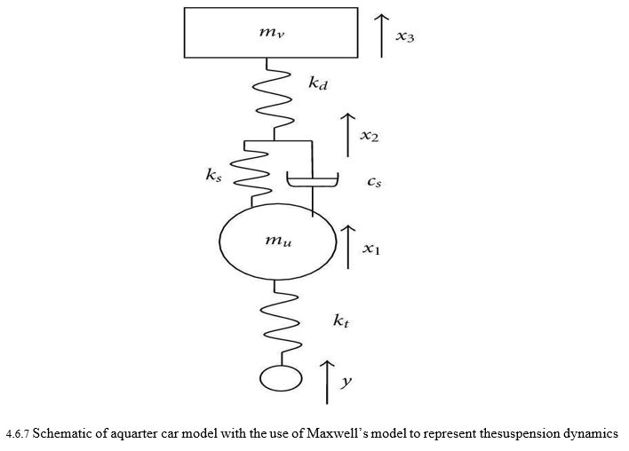
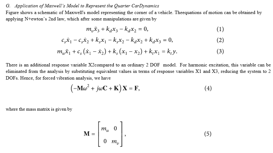
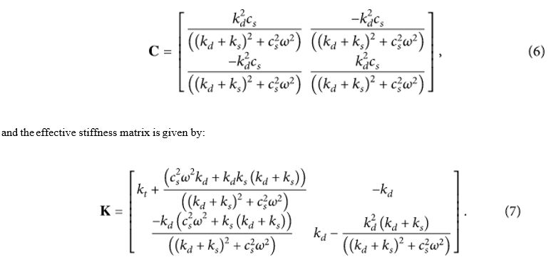
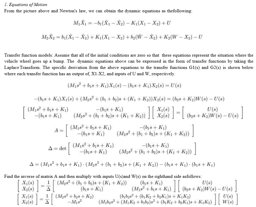
The elements of matrices are as follows: Mu is the effective mass of wheelMu hub, is a quarter of vehicle body mass, Cs is the suspension damping coefficient, Ks is the suspension stiffness, is the tire stiffness, is the series stiffness, Kt and is the excitation frequency. The stiffness matrix K has nonlinear elements; it is now dependent on the damping coefficient and excitation frequency. In the suspension system, for effective isolation at higher frequencies, the series spring stiffness is likely to be of the order of tire stiffness Kd [7] for a range of displacements; the effect on second resonance (the wheel hop frequency) is expected to be significant. The relative values of stiffness and damping coefficient determine the resonance frequency sensitivity. If the series stiffness is relatively large, the system would act as an ordinary two-DOF model and the spring and the damper being connected in parallel, irrespective of damping in the The effective damping (6) is also a complex function of series stiffness, suspension damping coefficient, and frequency, showing nonlinear behaviour. For large series stiffness values, it tends to the suspension damping coefficient. On the other hand, for small values, the damping is a complex function of series stiffness and frequency. The effective value determines the response peaks of the wheel hub and vehicle body motion. Later in this paper, an approximate expression is developed to estimate the optimum value of suspension damping coefficient.

Using (4), for a harmonic input, vehicle body and wheel hub responses can be calculated. The parameters used for the calculation are listed in Table 1, which can be obtained, for example, using the methods of [8]. Figure 2(a) shows wheel hub motion; there are two peaks, one each for the vehicle body bounce mode (around 2 Hz) and the wheel hop or hub mode (around 14 Hz). Also shown in the figure is the response where series stiffness is very large such that it can be treated as a rigid link. There is a significant difference in the response at the wheel hub frequency; the resonance is shifted and amplitudes are different. The vehicle body response also shows a similar pattern of behaviour (Figure 2(b)); the difference in wheel hub mode contribution to the response is more pronounced. The change in frequency and amplitude, as observed for the model with a series stiffness, can have significant influence on the vehicle comfort.

Vehicles went without suspensions for quite a long time. It was simply unnecessary at slow speeds. However, with the course of automobile industry development, increasing road quality and transporting speed there arose the need to increase transportation comfort. Let’s have a closer look at what is the suspension system, what are its construction features, functions and what types of suspension exist. Some background: how the first suspension appeared and construction improvement The first suspension looked rather primitive – details on long belts of leather or chains. When movement speed increased it tangibly decreased jumps and smoothened fluctuations of the compartment. Such a system was installed on caroches and post coaches. The scheme of modern suspension with bearings and elastic elements was developed by O. Elliott from England at the beginning of the 19th century. They used steel and wood for making shock absorbers. However, the item was still far from perfect and often broke on rough roads. They managed to overcome this defect as the metallurgy industry developed and made the suspension more rigid and load-resistant. Noticeably, such construction is still used in load-carrying trucks. The story of modern automotive suspension started in 1898. A French company named Deauville first used McPherson knee-action suspension with immovable bearings in a passenger car.

 Shock absorbers were first installed on automobiles in 1901. Mr. Mors, a Frenchman, installed them on a racing car as an experiment and in that very year, the race car driven by a racer A. Fourier won the race Paris-Berlin. Later in 1906 carriage springs were replaced by cylinder springs. Then during the 30s-50s construction engineers from all over the world worked on suspension improvement and tried every scheme of its construction and installation. From among all tested construction types the optimum ones were selected which are used by this day. Nowadays most passenger cars use suspensions of three types – independent construction, independent on double cross-installed levers, and semi-dependent with a torsion beam.

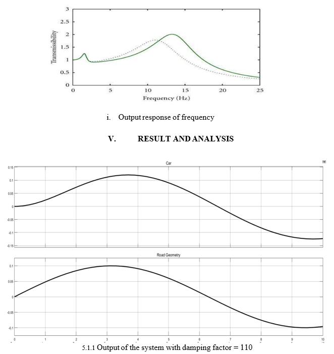
We give input as M=100 C= 110

K=10000 Y=0.1

F=0.5

Above parameter it will be give As input to the system the which will be give output As the change in damping factor 110 we observe relation between car geometry and road geometry it will be change and will increasing damping factor also change in car geometry

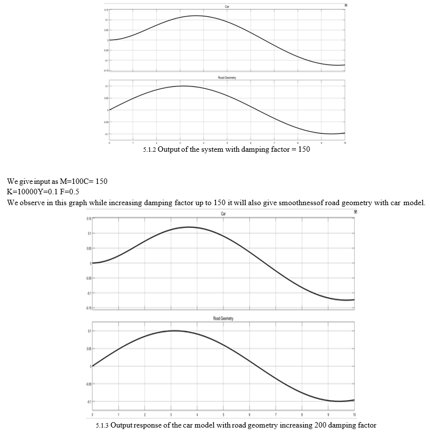
We give input as M=100 C= 200

K=10000 Y=0.1 F=0.5

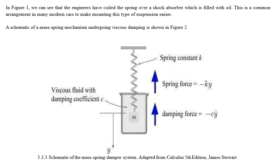
With changing damping factor with 200 Suspension damping is the process of controlling or stopping the spring's oscillation, either when it compresses or rebounds (usually both). By forcing the fluid through different size and shape ports, shims and tunnels, the damping cartridge can control the compression and rebound speed

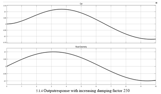
The ratio when increased from 110 to 250 1 (0 to 100%), will reduce the oscillations, with exactly no oscillations and best response at damping ratio equal to 1. On further increasing the damping ratio, the degree of damping has been overdone, this will cause sluggish performance/longer transients in the system.

Conclusion

A robust optimal control method is designed for the suspension system in order to improve the vehicle running performances, including handling stability and riding comfort. To address the uncertainties, including parameter perturbations and random road surface, the proposed optimal control method is designed by using the Matlab simulation optimal control and sliding-mode control. A collaborative simulation platform is developed. The simulation results illustrate that the proposed robust optimal controller not only can reach the optimal control objective but also has satisfactory robustness to the parameter uncertainty and external random disturbance.

References

[1] J. Na, Y. Huang, X. Wu, S.-F. Su, and G. Li, “Adaptive finite-time fuzzy control of nonlinear active suspension systems with input delay,” IEEE Trans. Cybern., vol. 50, no. 6, pp. 2639– 2650, Jun. 2020. [2] Y. Q. Xia, M. Y. Fu, C. M. Li, F. Pu, and Y. W. Xu, “Active disturbance rejection control for active suspension system of tracked vehicles with gun,” IEEE Trans. Ind. Electron., vol. 65, no. 5, pp. 4051–4060, May 2018. [3] Y. Li, P. Shi, and D. Y. Yao, “Adaptive sliding-mode control of Markov jump nonlinear systems with actuator faults,” IEEE Trans. Autom. Control, vol. 62, no. 4, pp. 1933–1939, Apr. 2017 [4] Y. Li, Z. X. Zhang, H. C. Yang, and X. P. Xie, “Adaptive event triggered fuzzy control for uncertain active suspension systems,” IEEE Trans. Cybern., vol. 49, no. 12, pp. 4388–4397, Dec. 2019. [5] Y.-J. Liu, Q. Zeng, S. C. Tong, C. L. P. Chen, and L. Liu, “Actuator failure compensation- based adaptive control of active suspension systems with prescribed performance,” IEEE Trans. Ind. Electron., vol. 67, no. 8, pp. 7044–7053, Aug. 2020. [6] Y.-J. Liu, Q. Zeng, S. C. Tong, C. L. P. Chen, and L. Liu, “Adaptive neural network control for active suspension systems with time-varying vertical displacement and speed constraints,” [7] IEEE Trans. Ind. Electron., vol. 66, no. 12, pp. 9458–9466, Dec. 2019 [8] X. Y. Zheng, H. Zhang, H. C. Yan, F.W. Yang, Z. P.Wang, and L. Vlacic, “Active full- vehicle suspension control via cloud-aided adaptive back stepping approach,” IEEE Trans. Cybern., vol. 50, no. 7, pp. 3113–3124, Jul. 2020. [9] R. Pradhan and B. Subudhi, “Double integral sliding mode MPPT control of a photovoltaic system,” IEEE Trans. Control Syst. Technol., vol. 24, no. 1, pp. 285–292, Jan. 2016 [10] M. A. M. Cheema, J. E. Fletcher, M. Farshadnia, and M. F. Rahman, “Sliding mode based combined speed and direct thrust force control of linear permanent magnet synchronous motors with first-order plus integral sliding condition,” IEEE Trans. Power Electron., vol. 34, no. 3, pp. 2526–2538, Mar. 2019. [11] G. P. Increment, M. Rubagotti, and A. Ferrara, “Sliding mode control of constrained nonlinear systems,” IEEE Trans. Autom. Control, vol. 62, no. 6, pp. 2965–2972, Jun. 2017. [12] Y.-J. Liu, S. C. Tong, C. L. P. Chen, and D.-J. Li, “Adaptive NN control using integral barrier Lyapunov functional for uncertain nonlinear block-triangular constraint systems,” IEEE Trans. Cybern., vol. 47, no. 11, pp. 3747–3757, Nov. 2017 [13] Y. B. Huang, J. Na, X.Wu, X. Liu, and Y. Guo, “Adaptive control of nonlinear uncertain active suspension systems with prescribed performance,” ISA Trans., vol. 54, no. 1, pp. 145– 155, 2015. [14] W. C. Sun, H. J. Gao, and O. Kaynak, “Adaptive backstepping control for active suspension systems with hard constraints,” IEEE/ASME Trans. Mechatron., vol. 18, no. 3, pp. 1072–1079, Jun. 2013.

Copyright

Copyright © 2022 More Akshay Narendra, Shakir Mufaddal Huzefa, Prof. Farheen Bobere . This is an open access article distributed under the Creative Commons Attribution License, which permits unrestricted use, distribution, and reproduction in any medium, provided the original work is properly cited.