Utilizing the HEC-HMS Model for Hydrological Modelling of the Rambiara Watershed: Rainfall and Runoff Estimation

Abstract

Hydrological modelling and flood prediction are essential components of the Rambiara watershed\'s water resource management. To improve disaster preparedness and reduce the danger of flooding in the area, the effectiveness of the HEC HMS model in flood forecasting must be assessed. In this study, various techniques for estimating rainfall are examined, and a customized hydrological model tailored to the hydrological complexities of the Rambiara watershed is developed. The goal of this project is to provide practical insights for better flood risk reduction and water resource management through the integration of cutting-edge modelling tools and rigorous analysis. This work advances our knowledge of watershed dynamics and provides guidance for sustainable water resource planning projects in the Rambiara watershed and beyond by thoroughly examining precipitation patterns and hydrological processes. In addition, the research takes into account a number of factors related to flood behaviour, such as determining places that are vulnerable to flooding, analysing the size of floods, and estimating how frequently they occur. By taking a holistic approach, it is possible to gain a thorough understanding of the dynamics of flooding in the Rambiara watershed, which paves the way for the development of efficient flood risk management techniques. This study looks into the temporal and spatial variability of rainfall in the Rambiara watershed in addition to research on floods. Through the comparison of several methods for estimating rainfall, including deterministic and geostatistical approaches, the study offers valuable insights into the precision and dependability of rainfall data, which are essential for hydrological modelling and flood forecasting. The hydrological processes of the Rambiara watershed can be more accurately represented by creating a bespoke hydrological model with the HEC HMS program. Informed decision-making and proactive flood risk reduction strategies are made possible by the study\'s model calibration and validation, which guarantee the model\'s dependability in simulating runoff and forecasting flood events. Overall, this study advances our knowledge of flood dynamics in the Rambiara watershed and advances hydrological modelling tools. The goal of this study is to promote sustainability and resilience in the face of hydrological hazards by offering practical insights for managing water resources and reducing the danger of flooding.

Introduction

I. INTRODUCTION

Water is the foundation of life on Earth and is necessary for all living things to survive. Ecosystems could not survive without water. But there's a serious problem with the growing demand for water due to things like intensive farming, population growth, urbanization, and poor management of available water resources. Water shortages brought on by this rising demand have a negative impact on ecosystems and human populations alike. Societies are left exposed and unable to fully recover from the effects of water scarcity, endangering livelihoods. Effective management planning is necessary to meet this challenge and maximize the use of the natural resources that are already accessible. In terms of developmental activities, the management of water resources and economic expansion are particularly important to the agricultural sector. The basic idea of hydrology, which offers the necessary framework for comprehending hydrological parameters and processes, is fundamental to the assessment and development of water resources. Stakeholders can ensure the resilience and prosperity of communities and ecosystems by developing policies for the sustainable management of water resources by utilizing hydrological knowledge.

A watershed is home to a complex web of hydrological processes that operate on various temporal and spatial scales. These activities include precipitation, interception, surface runoff, infiltration, groundwater percolation, and evapotranspiration. The way these elements interact results in the watershed's response, which is usually shown on runoff hydrographs. This reaction depends on a number of variables, including land use patterns, soil properties, rainfall characteristics, and human interventions. Watershed topography includes shape, size, slope, and orientation.

For example, if the land surface is parched after a dry summer, then heavy precipitation in the fall may not result in large runoff. The same precipitation, however, can cause floods in the winter or spring because the soils are wetter or have a higher moisture content, which allows for more surface runoff. In a similar vein, poorly managed agricultural methods can worsen erosion by introducing an excessive amount of fertilizers and pesticides into bodies of water, lowering the quality of the water within the watershed. High levels of complexity, nonlinearity, and spatiotemporal variability are seen in hydrological events. The mathematical depictions of catchment systems' reactions to hydrological events over predetermined time intervals are known as hydrological models. Not only do these models serve industrial demands but also human needs by analysing and forecasting streamflow, they are invaluable tools. To make the investigation easier, a popular model that works well in a variety of geographic contexts has been chosen for this study.

II. MATERIALS AND METHODS

This chapter outlines the selected study area, describes the data that was gathered and used for rainfall-runoff modelling, and provides an analysis of the models that were used. It focuses in particular on the calibration and procedure of the HEC-HMS model that is used to predict discharge at the Rambiara outlet within the watershed. Effective flood forecasting is the main goal. The following sections offer a thorough representation of the several datasets that were obtained throughout the study in order to successfully accomplish the goals of the research.

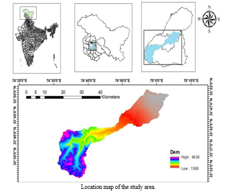
The Rambiara watershed, nestled within the picturesque locales of Shopian and Pulwama districts in Jammu and Kashmir, covers an area of 471 km². Originating from the lofty Rupri ridge of the Pir Panjal Range, the Rambiara River is nourished by the cascading waters from Rupri peak and the serene Bug Sar Lake on one side, and the mountain passes of Pir Panjal and Naba Pir on the other. Across its course, the river descends an impressive 2466 meters

The catchment area of the Rambiara spans approximately 75100 hectares, contributing significantly to the hydrology of the region. Its journey converges with the Vishu River before they both merge into the mighty Jhelum at Sangam, located at latitude 33°83 and longitude 75°07'. This confluence serves as a vital source of irrigation for the valley, sustaining agriculture and livelihoods

Situated amidst the left bank mountainous terrain of the Jhelum River in the western Himalayas, the Rambiara river basin occupies a strategic position between latitudes 33°33' and 33°54'N, and longitudes 74°30' and 75°00'E, enriching the southern region of Kashmir valley with its abundant natural resources.

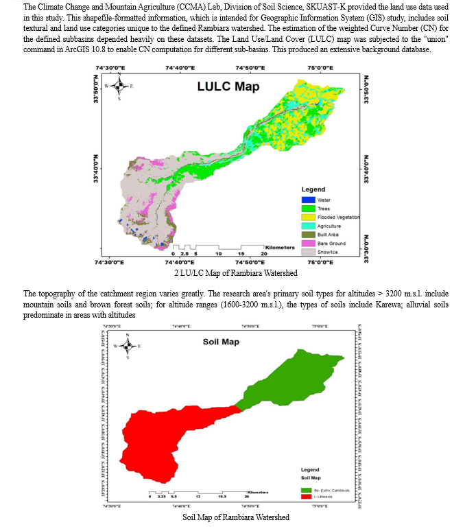
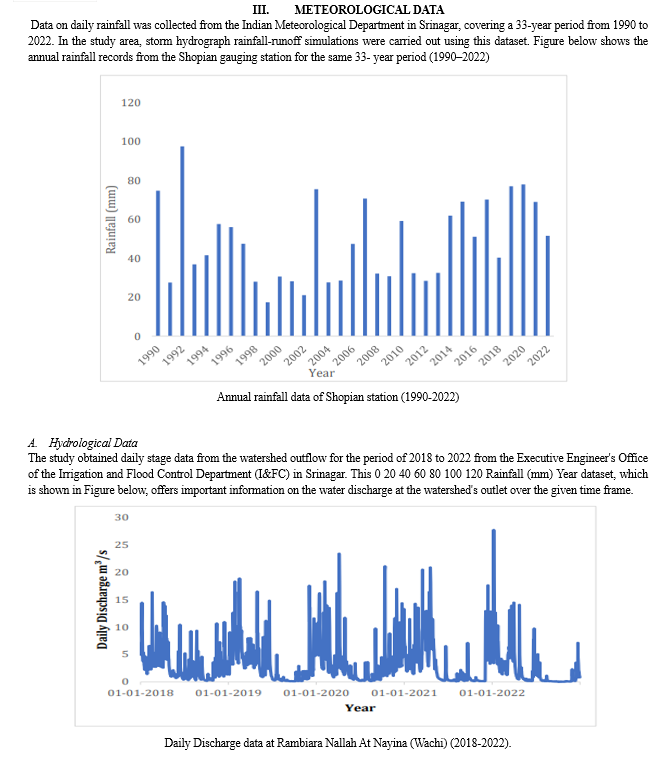
B. Estimation Of Mean Rainfall By Spatial Interpolation

As noted by Faure’s et al. (1995) and Chaubey et al. (1999), the use of point rain gauges for precipitation input causes substantial uncertainty in runoff estimation. Because of this uncertainty, it is difficult to anticipate discharge accurately, especially when rain gauges are located outside of the basin (Schuurmans and Bierkens, 2007). Hydrological modelling utilities require spatially continuous rainfall data in order to overcome these restrictions, as noted by Syed et al. (2003), Kobold and Sušelj (2005), Gabellani et al. (2007), Cole and Moore (2008), Collischonn et al. (2008), Ruelland et al. (2008), and Moulin et al. (2009). Singh (1997), Andréassian et al. (2001), Kobold and Sušelj (2005), Leander et al. (2008), and Moulin et al. (2009) have all 0 5 10 15 20 25 30 01-01-2018 01-01-2019 01-01-2020 01-01-2021 01-01-2022 Daily Discharge m³/s Year highlighted how much the quality of results depends on the spatial consistency of rainfall data.

Using known values from sampled points as a basis, spatial interpolation is a technique that predicts variable values at unsampled places. In order to estimate values at unknown places, a weighted average of the surrounding point values must be calculated. This process turns a discrete set of points into a continuous surface. The interpolated surface that is obtained is often known as a statistical surface, and it can be utilized for a variety of data types, including measurements of the groundwater table, elevation, temperature, precipitation, and snow accumulation. Waldo Tobler (1970) claimed that "Everything is related to everything else, but near things are more related than distant things" as the core tenet of interpolation. As a result, interpolation gives closer points a larger weight than farther points. Using GPS-measured elevation points to create a continuous map, such as a digital elevation map, requires the use of an appropriate interpolation technique to reliably predict values at places where samples or measurements are unavailable. Subsequently, the outcomes of interpolation analysis can be applied to more extensive area analyses and modelling. It's important to remember, though, that the variable should only be interpolated when it has a significant value at each location in the region of interest. Interpolation is not useful when points only show the existence of events without any associated values.

There are a number of difficulties in creating continuous surfaces from data that is unevenly distributed, especially when deciding which approach will best capture the true surface (Caruso and Quarta, 1998). Since the 1960s, there have been indirect methods for producing continuous surfaces from rainfall data by utilizing satellite platforms and ground-based meteorological RADARs. But more assessment is needed to determine the confidence and reliability of these indirect approaches for hydrological applications, which means historical data will need to be used for calibration and validation (Lanza et al., 2001). Many interpolation methods have been put forth in the literature to reproduce the spatial continuity of rainfall fields using rain gauge measurements. Deterministic approaches and geostatistical methods are the two primary divisions into which these techniques can be broadly divided. Deterministic approaches like Thiessen polygons and Inverse Distance Weighting (IDW) as well as geostatistical approaches like kriging are a few often employed strategies. The general formula for spatial interpolation is based on the idea that spatial interpolation usually entails estimating a regionalized value at unsampled places by giving weights to observed regionalized values.

Where:

Zg is the interpolated value at the required points;

Zsi is the observed value at point I;

ns is the total number of observed points and λ =

(λi) is the weight contributing to the interpolation.

The computation of the weights, λ, that will be applied to the interpolation presents a challenge. The next sections provide the various approaches used to calculate the weights and their results for the research area

IV. GEOSTATISTICAL METHODS

A. Kriging Method

The field of geo-statistics, which links mathematics and earth sciences, includes the first group of spatial interpolation methods for measuring rainfall. One such method is the Kriging method, which was named and formalized by Matheron (1971) in honor of Daniel G. Krige, a South African mining engineer who pioneered the field of geostatistics. Based on statistical models involving autocorrelation—that is, the statistical relationships between measured points—these methods can generate a prediction surface and provide measures of certainty and accuracy.

Using a weighted sum of the available point observations— selected to guarantee unbiased interpolation and minimize variance— Kriging estimates the value of the variable at a given point. Linear, Authorized, Unbiased, and Optimal (LAUO) systems are required for kriging. Kriging comes in various forms: Simple Kriging (SK), Ordinary Kriging (ORK), and Universal Kriging (UNK).

These variations are attributed to the form that is applied to the mean of the variable of interest. UNK is not stationary with respect to the mean, in contrast to the other methods, because it makes the assumption that the mean is a polynomial function of spatial coordinates

V. DETERMINISTIC METHODS

A. Nearest Neighbourhood method

The nearest neighbour (NN) approach, sometimes called the Thiessen polygon method, makes the assumption that calculated values can adopt the observed values of the closest station. Even though it is straightforward, the NN approach is regarded as sturdy and versatile, and it continues to be widely used even as more complex options emerge. This method involves selecting a predetermined number of data vectors that are comparable to the vector of interest, then randomly resampling one of those vectors to represent the vector for the current time step in the simulation period.

This entails simultaneously sampling and replacing weather variables from observed data, such as temperature and precipitation, in weather data simulation. Days having features akin to those simulated for the previous day are first chosen, and one of these nearest neighbour is then selected based on a specified probability distribution or kernel in order to create meteorological variables for a new day.

The next day's simulated values are based on the observed values for the day after that closest neighbour. While maintaining temporal and spatial connections, models built using the NN technique can be expanded to simulate meteorological data across multiple sites.

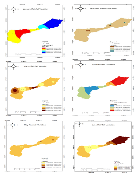
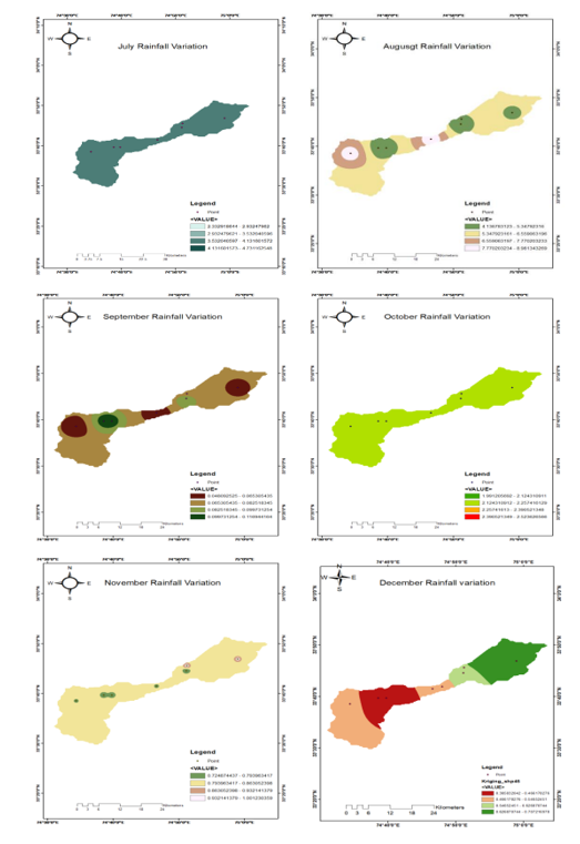
The weather of the same day is used for all stations, maintaining spatial dependencies, while each day's simulated values are predicated on the values from the day before, maintaining temporal reliance. Furthermore, when a block of variables rather than a single variable is resampled from observed data, cross-correlation among variables at any particular site is automatically retained. The research area's monthly rainfall interpolation map from January to December, produced using the nearest neighbour method

B. Performance Evaluation

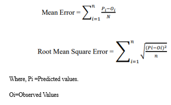
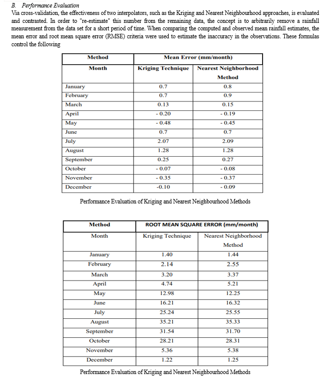
Using a strict cross-validation framework, we carefully assess and compare the performance of two well-known interpolators in this work: the Ordinary Kriging (OK) and Nearest Neighbour approaches. Our method consists of temporarily removing a rainfall observation that was chosen at random from the dataset, and then "re-estimating" the value of that observation using both interpolation techniques. We carefully check the estimated mean rainfall calculated using these techniques with the measured values. We use well-established measures, such as mean error and root mean square error (RMSE), to assess the quality of our estimations. A series of governing equations that have been carefully adapted to our study aims serve as the basis for these assessments. They are as follows:

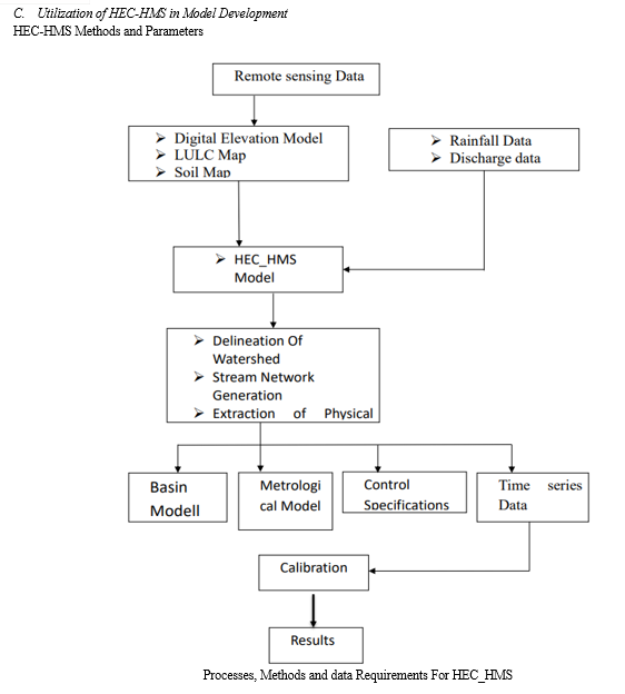
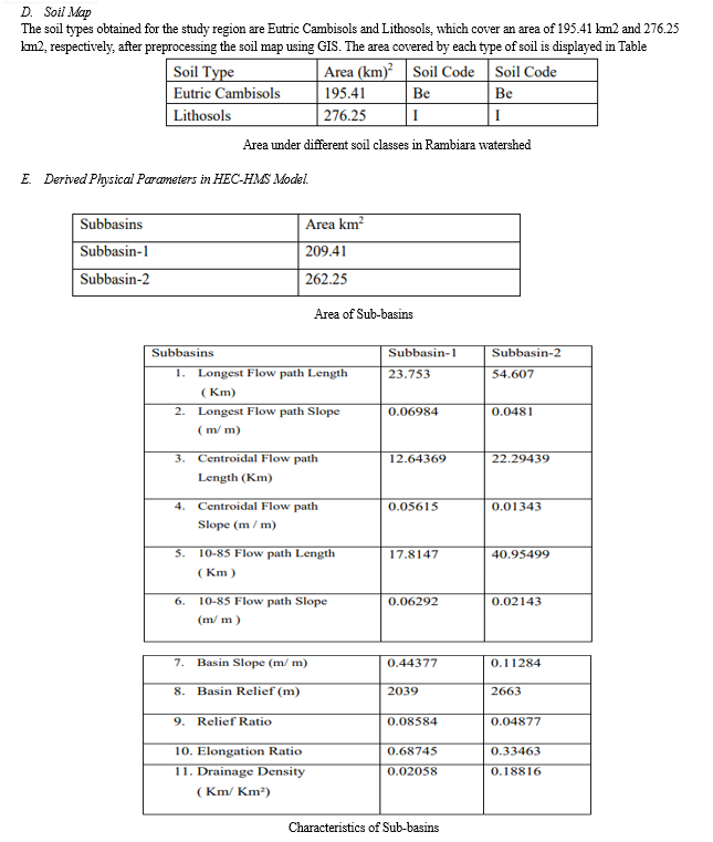
HEC-HMS is used to simulate precipitation-runoff processes, route flows across river networks, and assess hydrological responses in a simple way when developing models for watershed hydrology. In order to inform decisions about the management of water resources, this entails establishing the watershed, specifying hydrological parameters, choosing suitable models, executing simulations, and analysing the outcomes.

The hydrologic response of a watershed is simulated using the HEC-HMS model components. The primary elements are

• Basin model
• Meteorological model
• Control specifications and
• Time-Series Manager.

1. Basin Model: Determining the boundaries, topography, soil types, land use/cover, and hydrologic features (such as streams and reservoirs) of the watershed are all part of this component. The spatial distribution of hydrological parameters within the watershed is primarily represented by the basin model.
2. Meteorological Model: The hydrological model's incorporation of meteorological data is handled by the meteorological model component. This contains information on sun radiation, wind speed, temperature, humidity, and precipitation. The meteorological model provides inputs like rainfall and possible evapotranspiration, which assist drive the hydrological processes within the watershed.
3. Control Specification: Determining the simulation's characteristics and settings, including its duration, time step intervals, and other control options, is known as control specification. This part makes that the simulation performs in accordance with the intended goals and standards.
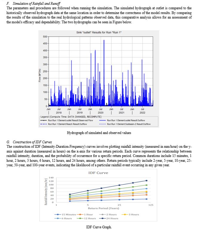
4. Time Series Data:  The historical or observable data used for model analysis, validation, and calibration is referred to as time series data. Measurements of streamflow, rainfall, and other pertinent hydrological observations gathered over time are usually included in this data. Time series data are necessary to verify the hydrological model's outputs against observed hydrological responses and assess the model's performance.

Deriving Physical Watershed Parameters

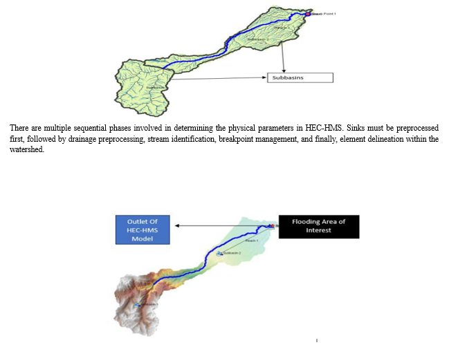
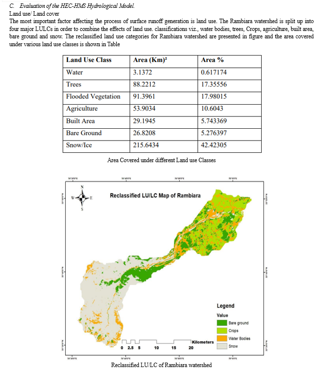
This section summarizes the findings of our study, which employed the HEC-HMS software to hydrologically model the Rambiara watershed, with a focus on rainfall estimation and flood forecasting. The study had three main goals: first, it estimated mean rainfall throughout the Rambiara watershed using a variety of deterministic and geostatistical techniques, such as nearest neighbourhood and Kriging techniques; second, it developed a hydrological model using the HECHMS software that was customized to the study area's features; and finally, it assessed the effectiveness of the HEC-HMS model in flood forecasting within the Rambiara watershed and improved the accuracy of flood predictions. In this section, we discuss the performance of several techniques for estimating rainfall, the creation and adjustment of the HEC-HMS model, and the evaluation of its efficacy in flood forecasting. The findings reported here help to enhance the region's capacity for flood prediction while providing insightful information on the hydrological dynamics of the Rambiara watershed.

A. Estimation of Mean Rainfall over the Rambiara Watershed Using Deterministic and Geostatistical Methods

The following figures display the monthly rainfall interpolation map of the research area from January to December produced by the nearest

Conclusion

Flooding is a major natural danger, which emphasizes how important it is to have trustworthy forecasting tools and safety precautions. It results from the buildup of surface runoff over a certain area, underscoring the critical need of precisely calculating runoff in order to properly forecast and minimize flood occurrences. The management of water resources and the operation of reservoir dams can be severely hampered by inaccurate runoff estimations. Therefore, using hydrological models to simulate rainfall-runoff processes becomes a practical way to estimate runoff. Utilizing hydrological models also makes it easier to comprehend the hydrological dynamics in catchment areas, which improves flood event preparedness and response tactics. The Rambiara watershed is located in the Indian Union Territory of Jammu and Kashmir. It is in a strategic location between latitudes 33°33\' and 33°54\'N and longitudes 74°30\' and 75°00\'E. This watershed, which is well-known for having an abundance of natural resources, is essential to improving the southern Kashmir valley. Using digital elevation models (DEM) and ArcGIS 10.8 and HEC-HMS 4.10, the Rambiara watershed was carefully mapped in this study. To achieve the study goals, a large dataset including daily discharge, rainfall, soil, and satellite data was gathered. The hydrological behaviour of the Rambiara watershed was investigated by a study that included HEC-HMS and previously published research. Then, in order to simulate streamflow dynamics, the HEC-HMS model was calibrated using rainfall and discharge data covering the years 2018 to 2022

References

[1] Fleming, M. (2004). Description of the hydrologic engineering center\'s hydrologic modelling system (HEC-HMS) and application to watershed studies. Atayi, M.A. 2017. Rainfall-Runoff Modelling Using Artificial Neural Networks and HEC-HMS (Case Study: Catchment of Gharasoo). International Journal of Engineering Research 6(7): 353-356. [2] Al-Abed, N., Abdulla, F. and Khyarah, A.A. 2005. GIS-hydrological models for managing water resources in the Zarqa River basin. Environmental Geology 47(3): 405-411. [3] Al-Zahrani, M., Al-Areeq, A. and Sharif, H. 2016. Flood analysis using HECRAS model: a case study for Hafr Al-Batin, Saudi Arabia. In E3S Web of Conferences 7: 04024. [4] Andr´eassian, V. Perrain, C. Michel, C. Usart-Sanchez, I. and Lavabre, J. (2001) “Impact of imperfect rainfall knowledge on efficiency and the parameters of watershed models” Journal of Hydrology, 250, 206–223. [5] Bhatt, A., Yadav, H. L., & Kumar, D. (2012). Estimation of infiltration parameter for Tehri Garhwal Catchment. International Journal of Engineering Research and Technology, 1(7), 1-6. [6] Caruso, C. and Quarta, F. (1998) “Interpolation methods comparison” Computers and Mathematics with Applications, 35(12), 109-126. [7] Chatterjee, M., De, R., Roy, D., Das, S., Mazumdar, A. and Bengal, W. 2014. Hydrological modeling studies with HEC-HMS for Damodar Basin, India. World Applied Sciences Journal 31(12): 2148-2154. [8] Chaubey, I. Haan, C.T. Grunwald, S. and Salisbury, J.M. (1999) “Uncertainty in the model parameters due to spatial variability of rainfall, Journal of Hydrology, 220(1-2), 48-61. Cole, [9] S. J. and Moore, R. J. (2008) “Hydrological modelling using raingage and radar-based estimators of areal rainfall” Journal of Hydrology, 358, 159– 181, 2008. [10] Collischonn, B. Collischonn, W. and Tucci, C. E. M. (2008) “Daily hydrological modeling in the Amazon basin using TRMM rainfall estimates” Journal of Hydrology, 360, 207–216, 2008. [11] Das, R. 2014. Study of Rainfall-Runoff Response of a Catchment using SCS Curve Number combined with Muskingum Routing Techniques. Structural and Civil Engineering. [12] Emerson, C.H., Welty, C. and Traver, R.G. 2005. Watershed-scale evaluation of a system of storm water detention basins. Journal of Hydrologic Engineering 10(3): 237-242. [13] Faur`es, J. M. Goodrich, D. C., Woolhiser, D. A, and Sorooshian, S. (1995) “Impact of small scale spatial variability on runoff modelling” Journal of Hydrology, 173, 309–326, 1995. [14] Gabellani, S., Boni, G., Ferraris, L., Hardenberg, J. V., and Provenzale, A. (2007) “Propagation of uncertainty from rainfall to runoff: A case study with a stochastic rainfall generator” Advances in Water Resources, 30, 2061–2071. [15] Goovaerts, P. (2000) “Geostatistical approaches for incorporating elevation into the spatial interpolation of rainfall” Journal of Hydrology, 228(1-2), 113-129. [16] Gautam, N. P. (2014). Flow routing with Semi-distributed hydrological model HEC-HMS in case of Narayani River Basin. Journal of the Institute of Engineering, 10(1). [17] Hutchinson, M.F. (1998) “Interpolation of rainfall data with thin plate smoothing splines-Part I: Two dimensional smoothing of data with short range correlation” Journal of Geographic Information and Decision Analysis, 2(2), 139-151. [18] Hofstra, N. Haylock, M. New, M. Jones, P. and Frei, C. (2008) “Comparison of six methods for the interpolation of daily, European climate data” Journal of Geophysical research, 113, 1- 19. [19] Karnieli, A. and Gurion, B. (1990) “Application of kriging technique to areal precipitation mapping in Arizona” Geojournal, 22(4), 391- 398. [20] Kastelec, D. and Kosmelj, K. (2002) “Spatial interpolation of mean yearly precipitation using universal kriging” Developments in Statistics, 149-162. [21] Kobold, M. and Su?selj, K. (2005) “Precipitation forecasts and their uncertainty as input into hydrological models” Hydrology and Earth System Sciences, 9, 322–332. [22] Kottek, M. and Rubel, F. (2008) “Co-kriging global daily rain gauge and satellite data” Geophysical Research, 10. [23] Kumar, D. and Bhattacharya, R. 2011. Distributed rainfall runoff modeling. International Journal of Earth Sciences and Engineering 4(6): 270-275. [24] Lanza, L.G. Ramirez, J.A. and Todini, E. (2001) “Stochastic rainfall interpolation and downscaling” Hydrology and Earth System Sciences, 5(2), 139-143. [25] Lloyd, C.D. (2005) “Assessing the effect of integrating elevation data into the estimation of monthly precipitation in Great Britain” Journal of Hydrology, 308(1-4), 128-150. [26] Matheron, G. (1971) “The theory of regionalized variables and its applications” Paris : École Nationale Supérieure des Mines de Paris. [27] McColl, C. and Aggett, G. 2007. Land-use forecasting and hydrologic model integration for improved land-use decision support. Journal of environmental management 84(4): 494-512. [28] Moulin, L. Gaume, E. and Obled, C. (2009) “Uncertainties on mean areal precipitation: assessment and impact on streamflow simulations” Hydrology and Earth System Sciences, 13, 99–114. [29] Nandalal, H.K. and Ratmayake, U.R. 2010. Event based modeling of a watershed using HEC-HMS. Engineer: Journal of the Institution of Engineers, Sri Lanka 43(2). [30] Nag, M., & Vishnu, B. (2013). Modelling the hydrology of watershed by using HEC-HMS (Doctoral dissertation, Department of Irrigation and Drainage Engineering). Naoum, S. and Tsanis, I.K. (2004) “Ranking spatial interpolation techniques using a GIS based DSS” Global Nest: the International Journal, 6(1), 1-20. [31] Parag, S. 2008. Rainfall-runoff modeling using HEC-HMS model. Unpublished B.Tech. thesis submitted to Deptt. of Irrig. and Drain. Engg., MPKV., Rahuri. Paudel, M., Nelson, E.J. and Scharffenberg, W. 2009. Comparison of lumped and quasi-distributed Clark runoff models using the SCS curve number equation. Journal of Hydrologic Engineering 14(10): 1098-1106. [32] Ravinder Kaur, R. K., & Dutta, D. (2002). GIS based digital delineation of watershed and its advantage over conventional manual method-a case study on watersheds in Hazaribagh and Bankura districts of Jharkhand and West Bengal. [33] Ripley, B. D. (1981) “Spatial statistics” John Wiley Sons, New York. Stewart, L. T., & Godchild, M. F. (1993). Integrating geographic information systems and environmental simulation models. Environ. Modeling With GIS, 16-30. [34] Schuurmans, J. M. and Bierkens, M. F. P. (2007) “Effect of spatial distribution of daily rainfall on interior catchment response of a distributed hydrological model, Hydrology and Earth System Sciences, 11, 677– 693. [35] Singh, V. P. (1997) “Effect of spatial and temporal variability in rainfall and watershed characteristics on stream flow hydrograph” Hydrological Processes, 11, 1649–1669. Syed, K. H. Goodrich, D. C. Myers, D. E. and Sorooshian, S. (2003) “Spatial characteristics of thunderstorm rainfall fields and their relation to runoff” Journal of Hydrology, 271, 1–21. [36] eteorology Vol, 11(22). Zhang, H.L., Wang, Y.J., Wang, Y.Q., Li, D.X. and Wang, X.K. 2013. The effect of watershed scale on HEC-HMS calibrated parameters: a case study in the Clear Creek watershed in Iowa, US. Hydrology and Earth System Sciences 17(7): 2735-2745

Copyright

Copyright © 2024 Dr. Bashir Ahmad Pandit. This is an open access article distributed under the Creative Commons Attribution License, which permits unrestricted use, distribution, and reproduction in any medium, provided the original work is properly cited.